
Posted on November 10, 2020 by Lisa Ward
by Doug Weaver
Last time we discussed the need to quantify everything in exploration, using my college glacial mapping project as an example. Let’s move back to the world of oil and gas exploration.
The main takeaway from my first blog is that an engineer’s role in exploration is to quantify. Geoscientists make interpretations of data and then engineers turn those interpretations into resource and economic assessments. The ultimate goal is to generate an inventory of opportunities that can be high-graded, allowing investment in those that are the most financially worthy. But how do we combine, resources, chance of success, costs, and economics to do this? We employ the expected value equation.
(Pc x Vc)-(Pf x Vf) = Expected Value
It’s a very simple equation. Let me describe the terms. Pc is the chance of success, Vc is the value of success. Pf is the chance of failure, Vf is the value (or cost) of failure. When we subtract the two terms we generate an expected value. If the expected value is positive the project is an investment candidate, if it’s negative, we’re gambling. We could still invest in a project with a negative expected value, but likely we’re going to lose money, and we’ll certainly lose if we invest in enough of them.
So let’s assume you’ve just generated a prospect, and you can make some estimate of a few items to describe it. You’ve got a rough idea of a chance of geologic success, maybe from working on a specific trend. You have some notion of size, either from your own volumetric assessment or again trend data. The engineer assisting your team with project evaluations should provide the team with a few key items to help with prospect screening.
- Threshold sizes – how big do prospects need to be to be commercial?
- NPV/Bbl (or Mcf) – what is the NPV/bbl for fields of various sizes? We’ll use this to transform barrels into dollars,
- Dry Hole cost – what is the dry hole cost for an exploration failure in the trend? (Might want to get depth specific here)
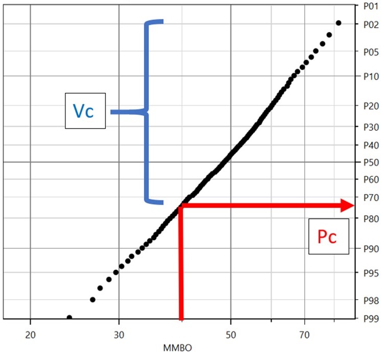
Back to the equation. First the success case. Notice both P (chance) and V (Value) in the success case have the subscript c, meaning commercial. What we’re looking for is the Commercial Chance and Commercial Value, not the geologic counterparts. If you have done a formal resource assessment this conversion is easy, you just determine where the threshold volume intersects the resource distribution. In the example below if the threshold is 40mmbo, it intersects the resource distribution at the 75th percentile. If this project has a geologic chance of success of 30%, the commercial chance of success is simply 30% x 75% or 22.5%. (For anyone not familiar with the convention, 40mmbo means 40 million barrels of oil).
The Commercial Volume would be determined by the resource that exists between the threshold volume and the maximum volume or between 40 mmbo and 76 mmbo. There are better ways to determine this, but for now let’s just use an average value of 58 mmbo.
Now you may ask, especially for screening, what if I don’t have this resource distribution? What if I’ve just made a quick deterministic volume estimate multiplying prospect area times a guess at thickness times a likely recovery yield (Bbl/ac-ft)? Can I still estimate the expected value? Sure, just try to apply the process described above as best you can. If the threshold is 40 mmbo and you calculate a resource of 300 mmbo, adjustments to geologic chance and volume will be minimal when considering their commercial values. If you calculate a volume of 45 mmbo, I might not try to estimate commercial values, but you already know the prospect is likely challenged commercially.
Now that we have an estimate of volume and chance, we need to convert our volume to value. The simplest way to do this is with a metric called NPV/bbl. The engineer assisting your team has likely evaluated many fields of various sizes in his evaluation efforts. Your group has probably generated other prospects in the trend, evaluated joint venture opportunities, and maybe even had a few discoveries.
For each of these opportunities the engineer has had to estimate the success case value or NPV (Net Present Value) for a given field volume, usually at the mean Expected Ultimate Resource(EUR). The NPV is going to account for the time value of money at your company’s specific discount rate. A typical discount rate is 10%, resulting in what is referred to as an NPV10. The NPV calculation accounts for all production (therefore revenue) and all costs and expenses over the life of the field, including the costs of completing the discovery well and drilling and completing appraisal wells, and reduces them to a single value. When this value is divided by the volume associated with the evaluation, we generate the metric in dollars/barrel of NPV/bbl. Given that these types of evaluations have been generated for several opportunities within a play, we can get a pretty good idea of how NPV/bbl changes with field size.
Note that for a given play in a given country NPV/bbl often doesn’t change dramatically. If you’ve only got a few field evaluations at your disposal the engineer should still be able to provide a usable NPV/bbl. Better yet embrace the uncertainty and test your prospect over a range of values. Finally, to determine Vc I simply need to multiply my mean EUR volume by my NPV/bbl.
The failure values are much easier to determine. Pf, the chance of failure is simply 1-Pc. Simple as that. For conventional exploration opportunities Vf or value (cost) of failure is usually just the dry hole cost. Most explorationists working on a trend have a pretty good idea of that cost, if not ask a drilling engineer. For the expected value equation, you should input an after-tax dry hole cost. Obviously, the tax rate will change from country to country, for the US the after-tax dry hole cost is about 70% of the actual cost.
Now we have all the pieces we need to generate the expected value. Let’s start with the plot earlier in this discussion and do that.
We have:
A commercial success volume of 58 mmbo
A commercial success chance of 22.5%
A failure chance of 77.5%
Let’s also assume an NPV/bbl of $2.00 and a dry hole cost of $20mm.
A couple of preliminary calculations
Value of success = 58mmbo x $2.00/bbl = $116mm
Cost of failure = $20mm x 0.7(tax) = $14mm
Here’s our equation
(Pc x Vc)-(Pf x Vf) = Expected Value
Plugging in values
(22.5% x $116mm)-(77.5% x $14mm) = Expected Value
$15,250,000 = Expected Value
Is this good? Yes, we’ve generated a positive value. Remember if it’s negative, we could still pursue the project but now we’re not investing we’re gambling. The key is that we need to perform this analysis on all our projects, look at our available funds, and invest in the best. That’s portfolio analysis and the topic of a later discussion.
The point of this blog was to simply walk you through the process, and encourage prospect generators to apply it to your opportunities as early as practical, even if it’s a “back of the envelope” calculation. Beyond chance and volume, all you need is a few values from your engineer. You’ll be able to use this tool to judge whether the prospect you’re working on is likely to be pursued or not. It may also give some insights as to what can be focused on to improve your prospect. For example, if you generate a low (or negative) expected value are there areas for improvement in chance or volume? If not, maybe it’s time to move on to the next one.