
Posted on November 10, 2021 by Lisa Ward
By Jim Gouveia, Marc Bond, Jeff Brown, Mark Golborne, Bob Otis, Henry S. Pettingill, and Doug Weaver
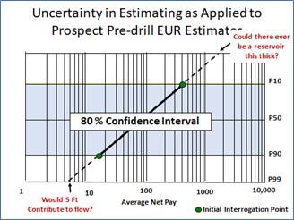
Consider the figure to the right under the lens of predicted net feet of pay. How have you been trained to handle plots such as this one? Here at R&A, we recommend a seven-step approach:
01. Plot the P10 and P90 predictions.
02. Draw a line between the predictions and extrapolate it to the resulting P1 and P99 values.
03. ‘Reality check’ these end members.
On the low end, would the predicted thickness contribute to meaningful sustainable flow? Assuming our area is unknown and highly correlated to our concept of sustainable flow, we get pragmatic and think about the ability to effectively complete the zone, without extraordinary measures. For example, would we be able to effectively complete a 1-foot interval in a homogenous sand which is underlain by 100 ft of water? There is no silver bullet for P99; it will be driven by user experience and play-specific knowledge, with consideration for variables such as permeability, Kv/Kh ratio, depth, infrastructure, viscosity, etc.
One of our biggest challenges when we consider net pay is defining how we differentiate geological successes from commercial successes. (We are talking about the average Net Pay across the productive trap area and not at the planned well location).
On the high end, could one make an optimistic yet realistic prospect map that could house such a thick Average Net Pay? In our collective experience at R&A, the projected P1 value can be unrealistically high—it’s not about the maximum thickness somewhere within the trap, it’s the maximum average thickness across the productive trap area.
04. Adjust the ‘reality check’ high and low members and pragmatically assume these are your new P1 and P99 end members.
05. Plot the ‘reality checked’ P1 and P99 values and redraw the line. The original P10 and P90 values are frequently not preserved and should be thought about as simply serving the purpose of initiating the process. Determine your resulting ‘reality checked’ P10, P50, and P90 values.
06. Inspect your measures of central tendency, the P50, and Mean values. For the P50, ask yourself, “When we think of this prospect, does it feel reasonable that half the time we expect to get a result larger than this value, and half the time less?” In a lognormal distribution, which best characterizes net pay, the P50 is halfway through the frequency, not halfway through the distribution’s parameter values. The Median, which is not synonymous with the P50, is based on sampled data. The reader is advised to always use the P50 which is based on the fitted data. When we are dealing with limited data sets, there can be a significant difference between the Median and the P50.
07. Compare the derived prospect Mean to the distribution of geologically analogous discovered prospects. Predicting a Mean outcome, which lies above the upper ten percent of your analogous discoveries, demands a technically unbiased explanation of why the prospect will have an Average Net Pay that exceeds 90% of the values previously encountered in the play.
Ultimately, exploration organizations need to deliver what they predict, and numerous industry look-back studies have demonstrated that the approach outlined in this example is highly effective in achieving that goal.
The values within our ‘reality checked’ P10 and P90 outcomes represent an “80% confidence interval.” In the E&P industry, we advocate setting the goal for our predictions based upon that range, particularly for the performance of our portfolios (more on that in a later R&A blog).
In a future blog, we will address measures of uncertainty and discuss reality checks based on our ratio of the P10 to P90.