Posted on March 18, 2021 by Lisa Ward
by Marc Bond, Senior Associate
Today I would like to talk with Creties Jenkins, co-creator of our Mitigating Bias, Blindness and Illusion in E&P Decision Making to gain another perspective on bias and how they impact our interpretations and decisions. Creties is a Partner at Rose & Associates with 35 years of diverse industry experience. As a geological engineer, he compliments my geoscience background.
Marc: Creties, welcome to my Understanding and Overcoming Bias blog. I appreciate you taking the time to give our readers some of your insights on our course.
Marc: I’d like to ask you what inspired you to put together the Mitigating Bias course.
Creties: First off Marc, thank you for the opportunity to provide some commentary for the bias blog. My primary inspiration for the Mitigating Bias course was Pete Rose’s AAPG Distinguished Lecture called “Cognitive Bias, the Elephant in the Living Room of Science and Professionalism”, which can be viewed on YouTube. He made the point that our lack of objectivity, due to errors in thinking, contributes to underperforming projects and portfolios. He also noted that the biggest challenge is convincing technical and management professionals that they are subject to bias, and concluded his talk by calling for a renewed commitment to the ‘rigor of the scientific method’. This is where our course picks up to provide some practical guidance.
Marc: In the course, we talk about Illusions. Can you give us some more insights?
Creties: We define an ‘Illusion’ as a misleading belief based on a false impression of reality. We focus on the Illusions of Potential, Knowledge, and Objectivity. Illusions are fueled by biases—we anchor on supporting data, we ignore disconfirming information, and we become overconfident in the expected result. My grandson, who’s a big superhero fan, was crushed when the Superman cape he ordered didn’t give him the ability to fly around the house. It never occurred to him that if this was real, friends and family members would already be using them. He was blinded by his own reality, which can happen to us as well.
Marc: Can you give an example?
Creties: All of us have seen Executive and Technical presentations touting the game-changing advantages of a given project, transaction or technology in our industry. We’ve come to expect that companies will overstate their knowledge and potential of these opportunities in order to generate investor buzz. But more importantly, we see companies believing their own press and not thinking critically enough about their proposed investments or having processes in-place to rigorously assess them and apply the lessons learned to new projects. The “Shale Revolution” in North America is a good example of companies repeatedly overpromising and underdelivering.
Marc: Do you see a relationship between Illusions and Cognitive Biases?
Creties: I do think that cognitive biases fuel illusions. We focus on small bits of data and analogs (information bias) that favor our intent (anchoring bias), ignore conflicting information (confirmation bias), convince us that our strategic plan is correct (framing bias) and that fame and glory will follow (motivational bias). So we think opportunities are better than they are (illusion of Potential), that we understand them more deeply than we do (illusion of Knowledge), and that we’re being honest and impartial in our resulting decisions (illusion of Objectivity). Without a constant awareness of this state and the application of mitigation techniques, we teach in our course, this sequence is all but certain to repeat itself. Just about every person reading this can recall at least one project in their company that followed this pattern with a disastrous result. And yet the cause and cure still receive scant attention.
Marc: What is one of your most surprising observations when teaching the course?
Creties: What’s most surprising to me is how few companies are interested in assembling case studies of their project failures and understanding the role that cognitive errors like ‘Illusions’ played. These case studies are really powerful because you have to admit that if a failure happened once in your company, it could happen again without some changes. I saw this first-hand at ARCO where the Illusion of Knowledge (mistaking familiarity for real understanding) led to a failed waterflood project because of unrecognized connected natural fractures. The inability to learn from this led a decade later to a billion-dollar failure of a miscible gas injection project for the same reason.
Marc: What is your biggest learning from teaching the course?
Creties: How prominent and impactful these cognitive errors are. We’ve presented this course nearly 100 times to everyone from field personnel to executives and nearly every attendee (based on course reviews) sees this problem within their company. Yet most companies are not addressing it or think it’s sufficient for personnel to simply have awareness. I did a half-day leadership version for one company and was told afterward that the attending geoscience managers favored a 2-day mitigation course for their reports, while the engineering managers favored a 1-day awareness course for their people. This led one of the geoscience managers to remark that geoscientists were interested in addressing the problem while the engineers were only interested in identifying it in others!
Marc: And could you leave us with a final message for our readers?
Creties: We provide our course attendees with an understanding of the different types of cognitive errors along with examples and steps to mitigate them in their daily work. But to create change, everyone in the organization needs to have a common vocabulary and processes (e.g., framing sessions, peer assists, performance lookbacks) that will expose and lessen the impact of cognitive errors. HR departments understand how these errors affect hiring, performance reviews, promotions, and employee interactions. We need the same recognition and desire for change on the technical side.
Check out more of Marc’s articles on bias and illusion on his LinkedIn profile.
Posted on February 24, 2021 by Lisa Ward
by Creties Jenkins, Partner
Quickly say the words in these three triangles.

If you didn’t pronounce the repeated words, you’re not alone. Nearly everyone fails to do so. But why? Our familiarity with these phrases causes us to predict the fourth word from the first three and ignore what’s in between. It demonstrates that events consistent with our expectations are processed easily while those that contradict them are ignored or distorted.
Our expectations have many diverse sources, including past experience, professional training, cultural norms, and organizational frameworks. These predispose us to pay particular attention to certain kinds of information and to organize and interpret it in certain ways. We are also influenced by the context in which information arises. Hearing footsteps behind you in the office hallway is very different from hearing them behind you in a dark alley!
These patterns of perception tell us subconsciously what to look for and how to interpret it. Without these patterns, it would be impossible to process the volume and complexity of data we receive every day. But we need to be aware of the downsides associated with these patterns:
01. Your view will be quick to form but resistant to change. Once you form an expectation for your project, this conditions your future perceptions.
02. New information will simply be assimilated into your existing view. Gradual, evolutionary change associated with new data often goes unnoticed, which is why a fresh set of eyes can reveal insights overlooked by someone working on the same project for many years.
03. Initial exposure to ambiguous information interferes with accurate perception. The greater the initial ambiguity, and/or the longer you’re exposed to it, the clearer the succeeding information must be before you’re willing to make or change an interpretation.
04. We tend to perceive what we expect to perceive. It takes more unambiguous information to recognize an unexpected outcome than an expected one.
05. Organizational pressures resist changing your view. Management values consistent interpretations, particularly those that promise added value to investors!
Fortunately, some techniques can help us overcome these downsides. We need to list our assumptions and chains of inference. We have to specify sources of uncertainty and quantify risk. Key problems should be examined periodically from the ground up. Alternative points of view should be encouraged and expounded.
These techniques, as well as others, are discussed and practiced in our Mitigating Bias, Blindness, and Illusion in E&P Decision-Making course. Please consider joining us for a virtual or in-person offering.
Reference excerpted for this blog: Heuer, Richard J., Jr., 1999, Psychology of Intelligence Analysis, Center for the Study of Intelligence.
Posted on February 17, 2021 by Lisa Ward
by Henry S. Pettingill, Marc Bond, Jeff Brown, Peter Carragher, Mark Golborne, Jim Gouveia, and Bob Otis
One of the common questions that teams ask us when reviewing subsurface projects is, “How should we set our input ranges for volumetrics?” This article introduces a new series that will address that question.
Many published works over the years have documented the importance of predicting what we find for our oil and gas portfolios, in both the exploration and development phases of the project life cycle. While it is impossible to repeatedly find exactly ‘the number’ for every prospect, well, or development, it is possible to get close the prediction on a portfolio basis. The fundamental concept is that for both prospects and portfolios, we can state our prediction in ranges, and additionally in terms of measures of central tendency (our ‘expectation’, commonly the arithmetic mean) and dispersion around that central tendency. The consequence of this latter statement is that we are able to give leadership ‘one number’ for an expectation – which is usually what both the executive suite and the investment community want from us.
So why do we use ranges? Simply put, it has been repeatedly shown that our predictions are better in the long run if, instead of using single values for each input parameter, we employ ranges to ultimately derive confidence intervals and a single value of our ‘expectation’ for that parameter (e.g. Pettingill, 2005). It also makes the elimination of systematic estimating bias more effective, as statistically rigorous post-mortem analyses become possible.
As far as we can tell, the pharmaceutical industry led the way in the 1920s by employing ranges in probabilistic predictions. The first employment of these methods in oil and gas volume prediction was documented in the late 1960s (for instance, Newendorp, 1968).
While most of the major upstream petroleum companies were employing these methods, they advanced and gained wider usage following seminal publications in the 1970s and 1980s by Ed Capen, Pete Rose, Bob Megill, Paul Newendorp, and others (see references below). These references have withstood the test of time and remain relevant today, so we highly recommend reading them.
Later works validated the concepts by demonstrating that pre-drill predictions as a whole were improved with the implementation of probabilistic ranges. These are well documented by Otis and Schneidermann (1997), Johns (1998), Ofstad et al. (2000), McMaster and Carragher (2003) and Pettingill (2005).
Fast forwarding to 2021, what have we observed over the years with respect to the application of these concepts? First, there are still many questions that arise on the topic from the upstream community. Second, some of the digital-era staff have not received an in-depth education on the fundamental concepts that drive input ranges. And finally, it seems like many of us who learned these methods have forgotten some of the fundamentals (or at least become rusty!).
Three fundamental concepts define the modern concepts for pre-drill volumetric assessment: 1) the jump from single deterministic input parameters to probabilistic inputs, 2) the use of continuous probability distributions (e.g., normal, lognormal), and 3) employing confidence intervals associated with these input distributions, and as a consequence, the final output distribution of recoverable resources.
These probabilistic ranges can be characterized by parameters such as probability percentiles (P10, P90, etc.), mean, variance or standard deviation, and P10:P90 ratios (Figure 1). We will expound on these in a future blog. [note: in this blog, we define P10 as high and P90 as low]. The biggest benefit from using these probabilistic ranges is the ability to state our predictions in terms of confidence, e.g. “I have a 90% chance of finding __ mmboe or greater, a 50% chance of getting __ mmboe or greater, and a 10% chance of getting __ mmboe or greater”. Another great advantage is the ability to characterize the distribution with a single mean value or the expectation that encompasses the entire output distribution: the mean, which is the average outcome. This allows us not only to understand the anticipated value of our portfolio as if we drilled our prospect thousands of times but also allows us to objectively compare and rank projects within a portfolio.
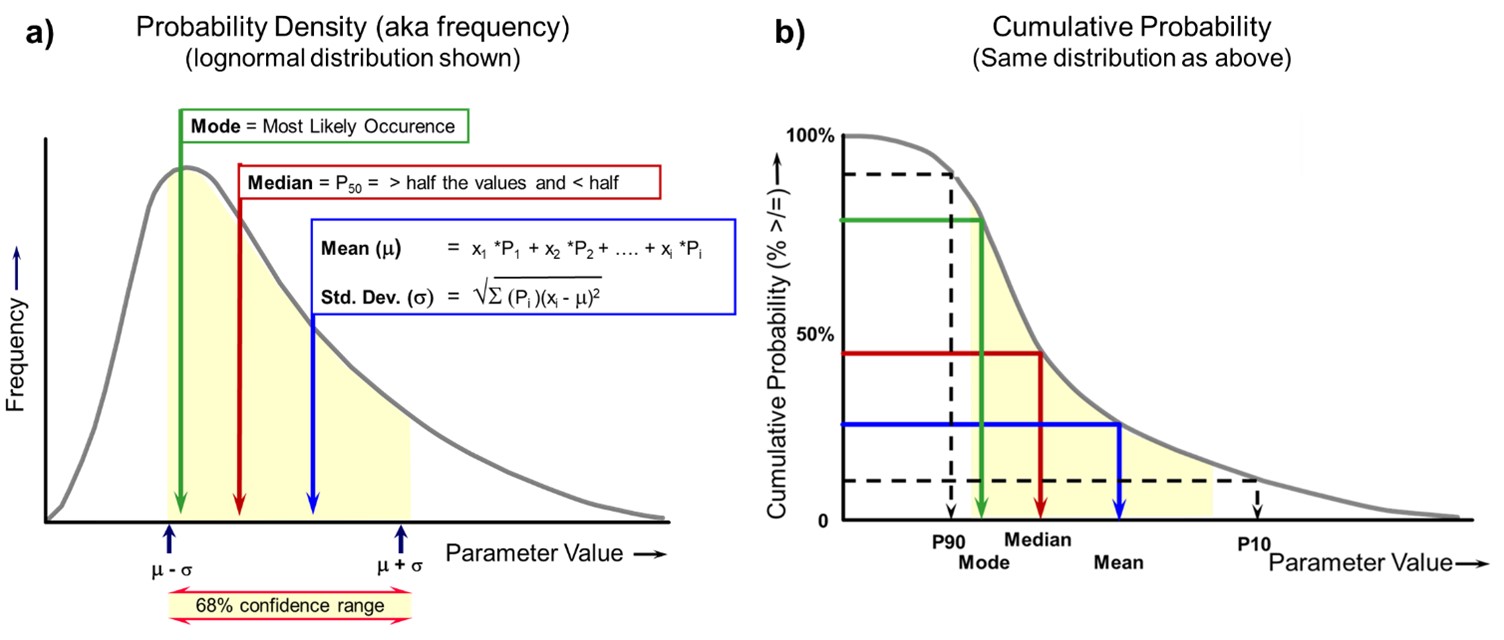
Figure 1. Probability graphs (lognormal distribution shown): a) probability density graph, b) cumulative probability graph. Note that we are using the “greater than or equal to” convention, with P90 as the low-end percentile. The concept applies to both the input parameter as well as the output distribution.
This series will evolve as we go along, so a precise schedule of topics is not set (of course, that will be driven largely by the comments from our readers!). Future topics being contemplated are:
— What should our modeled ranges represent?
— Different approaches to assessing uncertainty in Net Rock Volume (NRV)
— How to handle input parameters that use Averages (net pay, Phi, Sw, etc.)
— How to select ranges in the prospect area
— Spatial Concepts: how to jump from a map to a volumetric input distribution
— Direct Hydrocarbon Indicators (DHIs): specific considerations when choosing volumetric inputs
— Important statistical concepts: Mean, Variance, Standard Deviation, and P10/P90 ratios
We wish to thank all the authors of the works cited here, as well as the countless others not cited, for their contributions to this topic and our industry. They are the true heroes of this journey of learning. We also extend our gratitude to our colleagues at Rose and Associates.
— Capen, E. C. (1976), The difficulty of assessing uncertainty, Journal of Petroleum Technology, August 1976, pp. 843-850.
— Carragher, P. D. (1995), Exploration Decisions and the Learning Organization, Society of Exploration Geophysicists, August 1995, Rio de Janeiro.
— Johns, D. R., Squire, S. G., and Ryan, M. G. (1998), Measuring exploration performance and improving exploration predictions—with examples from Santos’ exploration program 1993-96, APPEA Journal, 1998, pp. 559-569.
— Megill, R. E. (1984), An Introduction to Risk Analysis, 2nd Edition. PennWell Publishing Co. Tulsa.
— Megill, R. E. (1992), Estimating prospect sizes, Chapter 6 in: R. Steinmetz, ed., The Business of Petroleum Exploration: AAPG Treatise of Petroleum Geology, Handbook of Petroleum Geology, pp. 63-69.
— McMaster, G. E. and Carragher, P. D. (1996), Risk Assessment and Portfolio Analysis: the Key to Exploration Success. 13th Petroleum Conference, Cairo Egypt, 1996.
— McMaster, G. E. and Carragher, P. D. (2003), Fourteen Years of Risk Assessment at Amoco and BP: A Retrospective Look at the Processes and Impact, Canadian Society of Petroleum Geologists / Canadian Society of Exploration Geophysicists 2003 Convention, Calgary Alberta, June 2-6.
— Newendorp, P. (1968). Risk analysis in drilling investment decisions. J. Petroleum Technology, Jun. pp. 579-85.
— Ofstad, K., Kittilsen, J.E., and Alexander-Marrack, P., eds. (2000), Improving the Exploration Process by Learning from the Past, Norwegian Petroleum Society (NPS) Special Publication no. 9. Elsevier, Amsterdam, 279 p.
— Otis, R. M., and Schneidermann, N. (1997), A Process for Evaluating Exploration Prospects, AAPG Bulletin v. 81, No. 7, pp 1087-1109.
— Pettingill, H.S. (2005) Delivering on Exploration through Integrated Portfolio Management: the Whole is not just the Sum of the Holes. SPE AAPG Forum, Delivering E&P Performance in the Face of Risk and Uncertainty: Best Practices and Barriers to Progress. Galveston, Texas, Feb. 20-24, 2005.
— Rose, P. R., (1987), Dealing with risk and uncertainty in exploration: how can we improve?, AAPG Bulletin, vol. 71, no. 1, pp. 1-16.
— Rose, P. R. (2000), Risk Analysis in Petroleum Exploration. American Association of Petroleum Geologists.
Posted on January 21, 2021 by Lisa Ward
by The Deep Coal Consortium (Deep Coal Technologies Pty Ltd, Rose & Associates, and Cutlass Exploration)
The Deep Coal Consortium is pleased to announce the completion of the first systematic review of the volumetric potential of the Gidgealpa Group Coal Measures in the deep portions (>3,000 feet) of the Cooper Basin based upon detailed analysis of well data (n=1,300). The Gidgealpa Group was evaluated in ten assessment intervals based on regional well correlation.
The study provides both deterministic and probabilistic estimates of in-place and technically recoverable gas and liquids, and (for the first time) Prospective Resources. Results are presented in tabular form and as a set of maps for each assessment interval and for the Group.
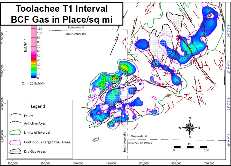
Low (P90), Median (P50), and High (P10) map realizations were generated for each assessment interval and volumes were aggregated to estimate the Group resource potential. An example of one interval is shown below.
The innovative methods used to calculate the map-based uncertainty in volumetric potential are discussed in URTEC 198304-MS.
The Deep Coal Play contains world-class volumes of potentially commercial gas and condensate. This volumetric study provides a strategic spatial context for decision-making as efforts to commercialize this play accelerate in the months ahead.
In addition, the data can be used to more fully characterize specific portions of the play, such as company acreage. The Consortium can provide technical support for such customized analysis.
For details contact David Warner of DCT.
Download this article as a PDF.
Posted on January 6, 2021 by Lisa Ward
by Henry Pettingill and Gary Citron
“It is amazing what you can accomplish if you do not care who gets the credit.”
Harry S. Truman
In 2000, a tipping point occurred when many companies wanted to see a consistent set of industry-derived best practices around amplitude characterization for a chance of success determination (prospect ‘risking’). In response, Rose & Associates’ founder Pete Rose and his Senior Associate Mike Anderson turned to former Shell and Maxus geophysicist and executive Mike Forrest to consistently weave seismic amplitude anomaly information into the fabric of prospect chance assessment. With the input of others, they decided to form a consortium of companies to capture best practices in a process that quickly evolved to include a user-friendly software and database, which became SAAM (‘Seismic Amplitude Analysis Module’). They reached out to Geologist Roger Holeywell, who was actively commercializing other risk analysis software for R&A through a partnership with his employer, Marathon Oil Corporation, to serve as SAAM programmer.
The DHI Consortium officially began at Dallas Love Field on December 7, 2000, a day recorded famously as the starting flag, with the inaugural meeting of the 13 founding companies in January 2001. Shortly thereafter Rocky Roden (Repsol’s Chief Geophysicist and representative to the first Consortium Phase, and a thought leader in geophysics) ‘retired’ from Maxus and joined Mike and Roger as the third director of the DHI Consortium.
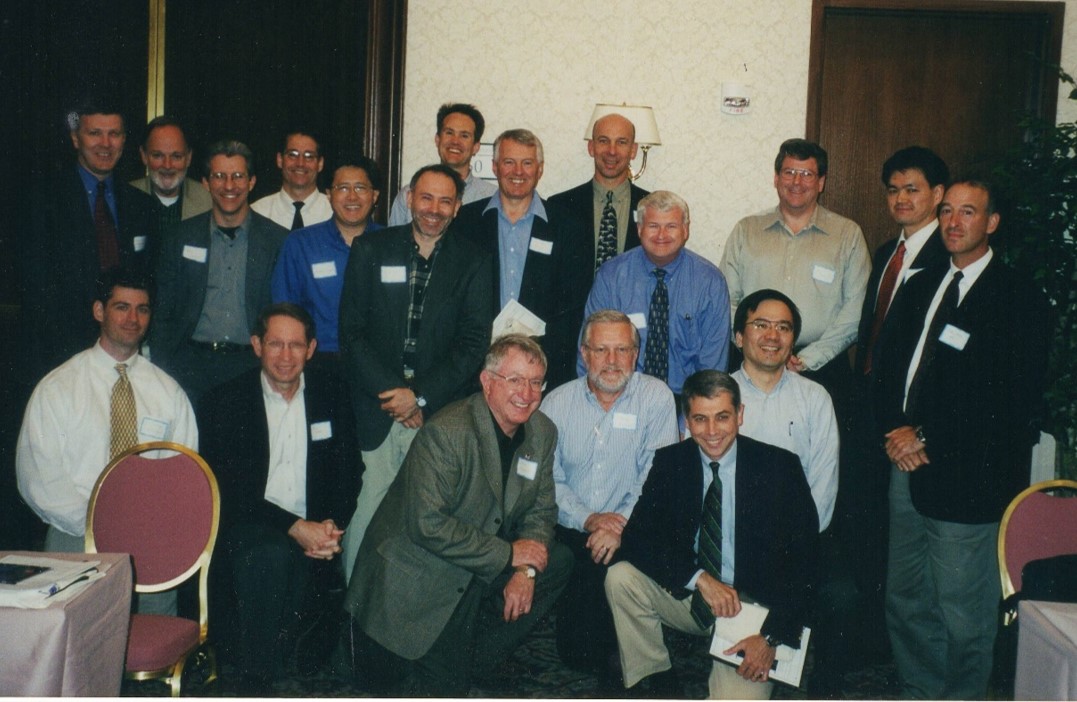
DHI Consortium group photo, May 2001 in Houston
In many basins with sandstone targets (especially those deposited during the Tertiary Period), the seismic signal associated with that target can be quite strong. Rock density and seismic velocity contrast noticeably between units, and that contrast is amplified by the presence of oil or gas in the pore system, making accumulations appear ‘anomalous’. The most common measure of the strength of the anomaly is the seismic amplitude (amount of signal deflection). These anomalies first became observable in the mid-1960s on relatively low-fold seismic lines and yielded significant quantifiable information as the fold increased.
While interpreting such seismic data, a geophysicist will measure an objective’s amplitude level in comparison to the ‘background’ level surrounding the objective amplitude. Significant amplitude strength above the background is referred to as an ‘anomaly’ or a ‘bright spot’. Mike Forrest is credited as one of the first explorers to recognize the exploration impact of seismic amplitude-bearing prospects when he was a Gulf of Mexico exploration project leader at Shell in the 1960s. The acronym DHI stands for Direct Hydrocarbon Indicator, suggesting that the seismic amplitude (hopefully) results from hydrocarbon charge.
At the very first meeting in January 2001, the Consortium commissioned Roger to program an innovative interrogation process that facilitates a thorough, systematic, and consistent grading of the amplitude anomaly, based purely on observations (as opposed to interpretations). It begins with the geologic setting, a preliminary chance assessment solely from geology (as if no DHI were present), and many key attributes the seismic data are designed to extract. SAAM requires the exploration team to answer questions about AVO classification, seismic data quality, rock property analysis, amplitude character, analogs, and potential pitfalls (also referred to as false positives). In other words, SAAM successfully institutionalizes a process through which explorers address salient issues, forcing those who would otherwise treat it in a perfunctory fashion to digitally record the key information they may later forget or lose. Employing a weighting system, SAAM registers the impact of each scored characteristic to determine a ‘DHI Index’, which in conjunction with the Initial Pg yields a ‘Final Pg’. This ‘Final Pg” is now calibrated by over 354 drilled wells.
Initially, each Consortium phase lasted 12 to 18 months. In 2016 Consortium phases were aligned with the calendar year to better synch with client budgeting. Consortium membership is paid through a phase fee and each new company that joins must purchase a license to SAAM. Companies may license a version of SAAM without joining the Consortium, but that version does not include the powerful analog and calibration database, which at the end of 2020 SAAM has 354 drilled prospects. The final Pg can then be analyzed in several ways, and critically compared to the success rates of similar DHIs and further calibrate the weighting system. SAAM’s burgeoning database is owned by Rose & Associates, with each member company having rights to internal usage.
In accepting AAPG’s highest honor in 2018 (the Sidney Powers award), Mike Forrest commented on the Consortium: “We expected it to last a year or two, and almost 20 years later it’s still going on!” Roger attributes the longevity to the breakthrough thought that meetings should be member-driven, designed around member company prospect presentations.
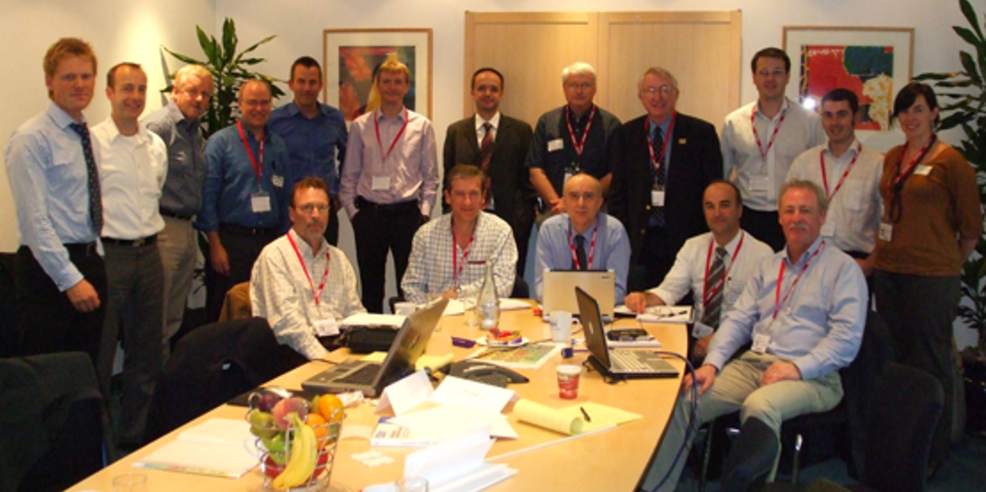
First European Chapter meeting, October 2007 in London
Can you think of any other venue to see drilled prospects, learn how they originated, how they were technically matured, the drilling outcome, and lessons learned from the journey – all within two hours? Companies benefit from seeing the tools and techniques other companies use in the analysis. Although some companies are unable to share the exact location of certain prospects, all the key attributes are shown and a SAAM file is populated for each prospect in real-time. Then the participants are asked for their opinions of prospect quality and ultimately whether they would drill it. The company then reveals the drilling results, and all inputs, outputs, and drilling results are added to the SAAM database.
As member participation in Consortium meetings grew, with more younger staff involved, the challenge became how to get more people in the room involved to avoid domination of discussion by senior members? Roger answered this question in 2017 by introducing the use of individual wireless keypads (’clickers’) that quickly register, compile, and display the entire group’s answers to a variety of grading questions anonymously. This permitted the leaders to ask people to explain their diverse views, which highlights how differing perspectives can get the discussion to a higher level.
SAAM’s architecture and workflow have constantly evolved but were always based on a collaborative framework. For every prospect shown in a meeting, during a subsequent weekend the Consortium Leadership gathered again to review the SAAM file, ensure consistency, and discuss what could be improved in the software, based on key observations from the prospect presentation.
Founding Consortium Chair Mike Forrest still consults with Consortium, which since 2019 has been under the direction of R&A’s Henry S. Pettingill. Henry was a member of the Consortium with Repsol during its inaugural year, and as Director of Exploration at Noble Energy, oversaw their participation since 2002. Roger and Rocky have guided and influenced the technical direction of the Consortium throughout its history. With companies opting in and out through the years, much of the stewardship of SAAM (updating functionality, testing, checking for consistency, and database trends) is left up to Roger’s discerning eye. He takes advantage of the crew changes, always on the lookout for the fresh perspective provided by new Consortium member feedback.
The Consortium’s secret sauce is relationships. That starts with the Leaders, who have known each other and worked together for over 20 years. Rocky and Henry both worked for Mike in the 1980s and 1990s at Maxus and Shell respectively, Rocky and Henry then worked together within Repsol/YPF Maxus. All along the way, Roger interacted with Mike, Rocky, and Henry, as authors of R&A’s software products.
But there is also a strong bond between many of the members, some of whom have interacted in and out of the Consortium for over 20 years. One of the highlights of Consortium meetings in Europe is the way each host company highlights the unique aspects and special history of their city and culture through a ‘networking dinner’ featuring the local cuisine. These became an instant tradition, strengthening the network by building friendships amongst the industry’s elite DHI practitioners. There have even been occasional field trips to classic locations in Europe and South Africa.
Each year, the Consortium typically holds five meetings in Houston and three in Europe. Since March 2020, due to the COVID-19 pandemic, the meetings were replaced by monthly webinars. This turned out to be a blessing in disguise as it caused a surge in participation and expanded the reach of the Consortium. Whereas most people can attend a meeting only occasionally (and those in remote field offices virtually never), webinar attendance far exceeded regular meeting attendance, with new participation from field offices in the Netherlands, Oman, Malaysia, Indonesia, and New Zealand.
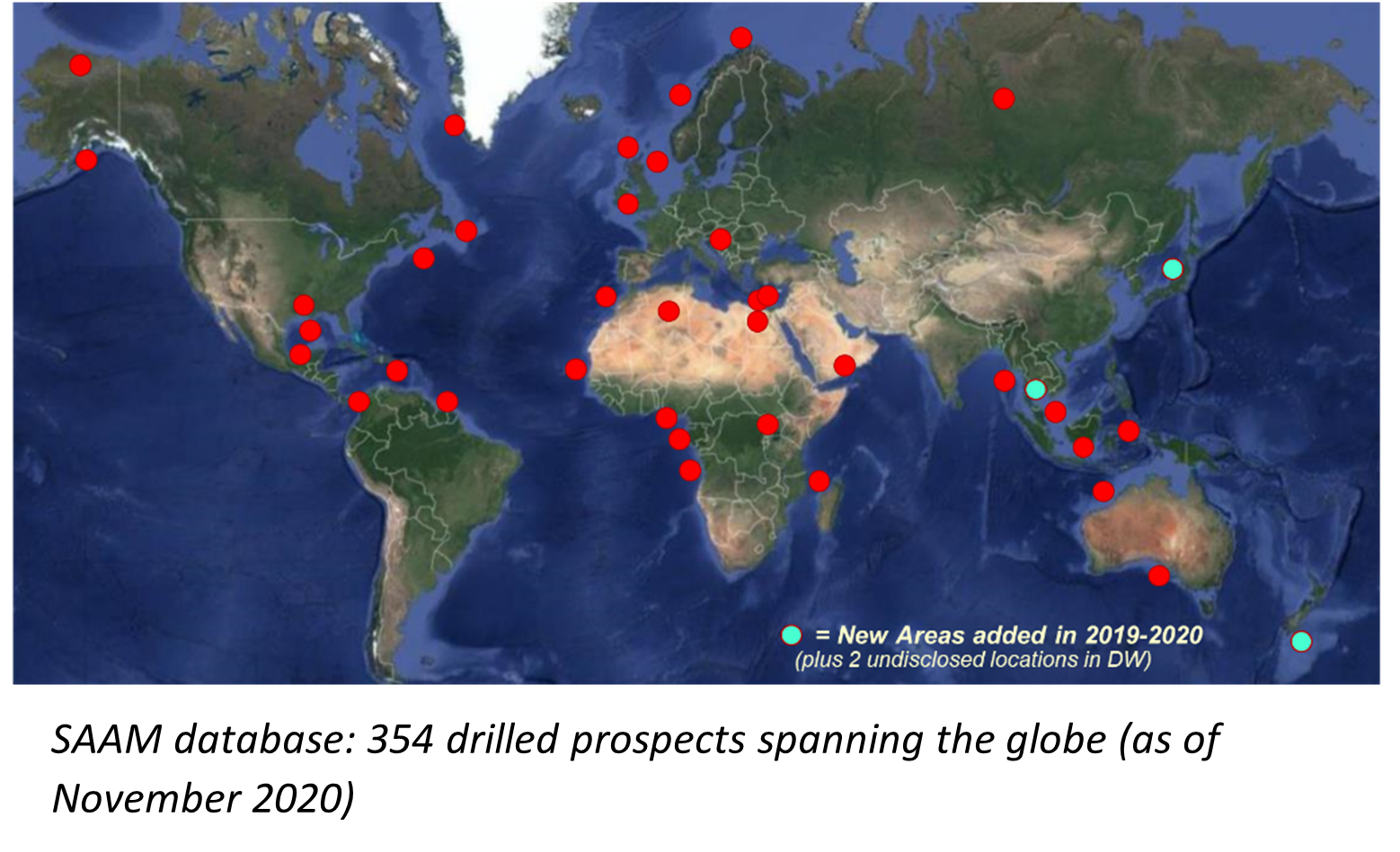
As we celebrated our 20th anniversary in this month’s webinar, we looked back on the 20 years and some of its accomplishments – too many to list here. In numbers, the SAAM database has 354 drilled prospects from 30 basins, allowing calibration of assessments of undrilled prospects, as well as providing valuable benchmarking data. Over 80 companies have participated, most of whom have contributed drilled prospects to the database, and we have 36 member companies this year. But probably the most enduring accomplishment is the heightened prospecting skills and intuition of the participants. This has resulted in the Industry’s most comprehensive DHI prospect database, all evaluated using consistent methodology and peer-reviewed by a roomful of advanced practitioners.
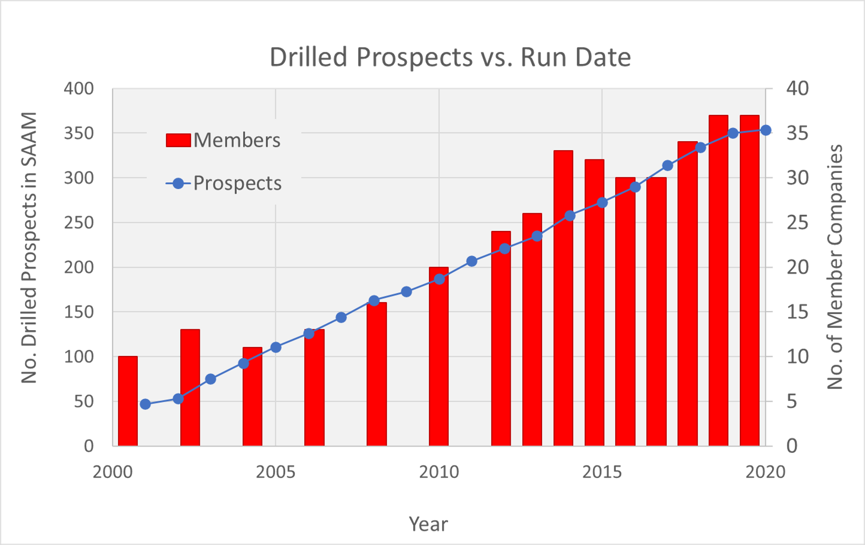
Consortium membership and SAAM database vs. time
Perhaps most remarkable is how the Consortium has evolved with time and technology. For instance, seismic imaging and other advances have allowed for things unthinkable just a few years ago, like imaging amplitudes beneath salt. Computer power and machine learning have allowed analyses like never before. And each year, the Consortium sets goals according to where we are in this evolution.
It all leads us to ask: what will the next 20 years have in store for us? Most of us agree that changes will continue to come in DHIs and associated exploration technologies, and make the unimaginable not just imaginable, but even more fun.
Posted on December 9, 2020 by Lisa Ward
by Marc Bond
Following a groundswell of interest generated by a presentation at the 2008 AAPG Annual Convention by Glenn McMaster et al entitled “Risk Police: Evil Naysayers or Exploration Best Practice?” several (including myself, then at BG Group) thought it would be an excellent idea to organize a workshop to discuss best practices and challenges of exploration assurance. Glenn (then at bp) was great at speaking truth to power and embraced the idea. Hence, he and Gary Citron (at Rose & Associates) convened the first Risk Coordinators Workshop (RCW) on November 18-19, 2008, graciously hosted by bp in Houston. Twenty-eight industry leaders from 18 companies attended. Twelve presentations were given by the attendees, mostly focused on the state of assurance within the company of the presenter which was a rare insight at the time. That openness fostered a sharing and collaborative environment, defusing our concern that this would be a “one-off “event. Rather, the enthusiasm and interest of the successful workshop encouraged us to continue.
I particularly enjoyed attending and contributing to the Workshop through the years. We now continue with a yearly workshop, with the goal of sharing common experiences, issues, challenges, and suggested best practices. There is a nominal fee for attendees to cover expenses. The only obligation is to be open and share. We held our 19th annual workshop in November 2020. Given the current situation of the pandemic, the RCW was held virtually for the first time; and measured by the commentary and feedback, was a great success.
When I joined Rose & Associates in 2014, I brought in the idea of increasing workshop frequency, and we now meet two to three times a year (in North America and England, and every other year in Asia). We also now include Breakout Sessions to explore relevant assurance themes and provide a Summary Report to capture the outcomes of each workshop.
In 2015, we established the Risk Coordinators network as a natural follow-up to the RCW, which consists of a group of subsurface assurance experts who are responsible for assuring their companies’ opportunities. The network is an informal group that includes over 70 companies (ranging from super-majors to small companies) and over 160 people who are very open and passionate about assurance, risk analysis, and prospect assessment. Along with the workshops, we have now been active for over 12 years.
We work with the network on other assurance-related items, such as delivering a periodic Assurance Survey (2015 and 2019). The Survey results are shared with the network to monitor the current state of assurance and provide them with learnings to help improve their own assurance process.
Doug Weaver (Partner Rose & Associates) and I now manage the network. I would like to personally thank Gary for his support and coaching over the years. If you have any questions about the network or ideas for the next RCW, please contact us
Stay safe and healthy.
Posted on November 10, 2020 by Lisa Ward
by Doug Weaver
Last time we discussed the need to quantify everything in exploration, using my college glacial mapping project as an example. Let’s move back to the world of oil and gas exploration.
The main takeaway from my first blog is that an engineer’s role in exploration is to quantify. Geoscientists make interpretations of data and then engineers turn those interpretations into resource and economic assessments. The ultimate goal is to generate an inventory of opportunities that can be high-graded, allowing investment in those that are the most financially worthy. But how do we combine, resources, chance of success, costs, and economics to do this? We employ the expected value equation.
(Pc x Vc)-(Pf x Vf) = Expected Value
It’s a very simple equation. Let me describe the terms. Pc is the chance of success, Vc is the value of success. Pf is the chance of failure, Vf is the value (or cost) of failure. When we subtract the two terms we generate an expected value. If the expected value is positive the project is an investment candidate, if it’s negative, we’re gambling. We could still invest in a project with a negative expected value, but likely we’re going to lose money, and we’ll certainly lose if we invest in enough of them.
So let’s assume you’ve just generated a prospect, and you can make some estimate of a few items to describe it. You’ve got a rough idea of a chance of geologic success, maybe from working on a specific trend. You have some notion of size, either from your own volumetric assessment or again trend data. The engineer assisting your team with project evaluations should provide the team with a few key items to help with prospect screening.
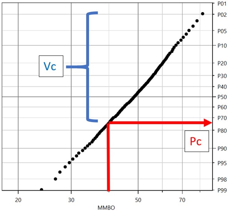
Back to the equation. First the success case. Notice both P (chance) and V (Value) in the success case have the subscript c, meaning commercial. What we’re looking for is the Commercial Chance and Commercial Value, not the geologic counterparts. If you have done a formal resource assessment this conversion is easy, you just determine where the threshold volume intersects the resource distribution. In the example below if the threshold is 40mmbo, it intersects the resource distribution at the 75th percentile. If this project has a geologic chance of success of 30%, the commercial chance of success is simply 30% x 75% or 22.5%. (For anyone not familiar with the convention, 40mmbo means 40 million barrels of oil).
The Commercial Volume would be determined by the resource that exists between the threshold volume and the maximum volume or between 40 mmbo and 76 mmbo. There are better ways to determine this, but for now let’s just use an average value of 58 mmbo.
Now you may ask, especially for screening, what if I don’t have this resource distribution? What if I’ve just made a quick deterministic volume estimate multiplying prospect area times a guess at thickness times a likely recovery yield (Bbl/ac-ft)? Can I still estimate the expected value? Sure, just try to apply the process described above as best you can. If the threshold is 40 mmbo and you calculate a resource of 300 mmbo, adjustments to geologic chance and volume will be minimal when considering their commercial values. If you calculate a volume of 45 mmbo, I might not try to estimate commercial values, but you already know the prospect is likely challenged commercially.
Now that we have an estimate of volume and chance, we need to convert our volume to value. The simplest way to do this is with a metric called NPV/bbl. The engineer assisting your team has likely evaluated many fields of various sizes in his evaluation efforts. Your group has probably generated other prospects in the trend, evaluated joint venture opportunities, and maybe even had a few discoveries.
For each of these opportunities the engineer has had to estimate the success case value or NPV (Net Present Value) for a given field volume, usually at the mean Expected Ultimate Resource(EUR). The NPV is going to account for the time value of money at your company’s specific discount rate. A typical discount rate is 10%, resulting in what is referred to as an NPV10. The NPV calculation accounts for all production (therefore revenue) and all costs and expenses over the life of the field, including the costs of completing the discovery well and drilling and completing appraisal wells, and reduces them to a single value. When this value is divided by the volume associated with the evaluation, we generate the metric in dollars/barrel of NPV/bbl. Given that these types of evaluations have been generated for several opportunities within a play, we can get a pretty good idea of how NPV/bbl changes with field size.
Note that for a given play in a given country NPV/bbl often doesn’t change dramatically. If you’ve only got a few field evaluations at your disposal the engineer should still be able to provide a usable NPV/bbl. Better yet embrace the uncertainty and test your prospect over a range of values. Finally, to determine Vc I simply need to multiply my mean EUR volume by my NPV/bbl.
The failure values are much easier to determine. Pf, the chance of failure is simply 1-Pc. Simple as that. For conventional exploration opportunities Vf or value (cost) of failure is usually just the dry hole cost. Most explorationists working on a trend have a pretty good idea of that cost, if not ask a drilling engineer. For the expected value equation, you should input an after-tax dry hole cost. Obviously, the tax rate will change from country to country, for the US the after-tax dry hole cost is about 70% of the actual cost.
Now we have all the pieces we need to generate the expected value. Let’s start with the plot earlier in this discussion and do that.
We have:
A commercial success volume of 58 mmbo
A commercial success chance of 22.5%
A failure chance of 77.5%
Let’s also assume an NPV/bbl of $2.00 and a dry hole cost of $20mm.
A couple of preliminary calculations
Value of success = 58mmbo x $2.00/bbl = $116mm
Cost of failure = $20mm x 0.7(tax) = $14mm
Here’s our equation
(Pc x Vc)-(Pf x Vf) = Expected Value
Plugging in values
(22.5% x $116mm)-(77.5% x $14mm) = Expected Value
$15,250,000 = Expected Value
Is this good? Yes, we’ve generated a positive value. Remember if it’s negative, we could still pursue the project but now we’re not investing we’re gambling. The key is that we need to perform this analysis on all our projects, look at our available funds, and invest in the best. That’s portfolio analysis and the topic of a later discussion.
The point of this blog was to simply walk you through the process, and encourage prospect generators to apply it to your opportunities as early as practical, even if it’s a “back of the envelope” calculation. Beyond chance and volume, all you need is a few values from your engineer. You’ll be able to use this tool to judge whether the prospect you’re working on is likely to be pursued or not. It may also give some insights as to what can be focused on to improve your prospect. For example, if you generate a low (or negative) expected value are there areas for improvement in chance or volume? If not, maybe it’s time to move on to the next one.
Posted on September 30, 2020 by Lisa Ward
by Marc Bond, Senior Associate
Success and value creation in the oil and gas industry have not been particularly good, as evidenced by its relative performance. This is widely recognized both in the global markets and within the industry itself. There are certainly many reasons that may explain why the oil and gas industry has not done well over the years, and one area that has received a lot of traction in recent years is the concept of cognitive bias.
Cognitive biases are predictable, consistent, and repeatable mental errors in our thinking and processing of information that can, and often do, lead to illogical or irrational judgments or decisions.
Surprisingly, the notion of cognitive bias has not been around for many years. It was first proposed by Amos Tversky and Daniel Kahneman in 1974 in an article in Science Magazine (Tversky and Kahneman, 1974). Since then, there have been numerous publications and research studies on the various cognitive biases and how they impact our judgments and decisions.
The book that introduced the concept of cognitive biases and their influence on the decisions of the general population was the seminal publication by Nobel Prize-winning psychologist Daniel Kahneman – Thinking, Fast and Slow (Kahneman, 2011). It is interesting to note that Dr. Kahneman won the Nobel Prize in 2002 not in Psychology, but rather in Economics. Why? Because traditional economic theory assumes that we are rational creatures when we make decisions or choices, and yet research and observations continually show that we do not.
There are many different cognitive biases (see Wikipedia), but there are a few that play a significant role within the oil and gas industry. These biases can act individually or in combination, leading us to poor judgments and decisions.
For example, imagine an exploration team is assessing a prospective area that is available for license bids. In the analysis of the data, the focus is on a very productive analog to describe the play. Nearby there has been a successful well recently drilled; and although it is acknowledged to be in a different play, the team is very excited about the hydrocarbon potential of their new play.
Some existing, older wells suggest that the new play may not work, but it is felt by the technical team that those wells were either old or poorly completed, and hence could be dismissed as valid data points. Given the uncertainty, the prospects and leads developed should have a very wide range of resource potential. However, given the team’s confidence in the seismic amplitudes, the range of GRVs estimated is quite narrow.
The team is also optimistic about the play potential and presents the opportunity to management in very favorable terms. If the company were to bid on and be awarded the license by the government, the team would be quite excited; and of course, success is often rewarded. The company ended up bidding on the license with a commitment of several firm wells. Upon further data collection and data analysis, a new team re-assessed the hydrocarbon potential and it is now believed to be limited; and yet there still is a large commitment to fulfill.
What happened to cause this result? Was the original team overconfident in their expectations? Did they think that because they understood their commercial analog, they understood the perspective? Were they so focused on the nearby successes? Was the data that was dismissed highly relevant? Were other alternatives and models not considered, which might have suggested that the resource size could be small?
Although the above narrative may appear to be contrived and one’s reaction to the scenario would probably be “I would never do that”, each of the justifications and decisions made are possibilities and all of them are rooted in forms of cognitive bias. You likely have recognized all or part of the scenario from your own experience. Further, these biases can work together in a complementary fashion, reinforcing the biased assessment, and making one “blind” to other possibilities.
Cognitive biases and their negative impact do not just present themselves during the exploration phase. There are numerous similar real-world scenarios observed in appraisal, development, production, and project planning projects.
The bottom line is that these cognitive errors lead to poor decisions regarding work to undertake, issues to focus on, and whether to forge ahead or exit a project. This makes it important to identify them and lessen their impact. Unfortunately, awareness alone is not sufficient. These biases are inherent in our judgments and decision-making and serve the purpose of helping us make rapid judgments based on intuition and experience. In our everyday life, they work generally well. Unfortunately, particularly in complex and uncertain environments such as the oil and gas industry, they can lead us to poor choices.
Hence, it is important to understand first what the biases are, why they occur, and how they can influence our assessments. This will then help us identify when our own, or our colleague’s judgments, assessments, and decisions may be affected by these cognitive biases. We then need to learn mitigation strategies. Given that these cognitive biases are normal and serve a purpose, the goal cannot be to remove them but rather to recognize the biases and then apply mitigation strategies to lessen their impact.
As noted above, there has been a lot of research on the biases, yet there is little published on actual, practical mitigation strategies. Hence, to help our industry, my colleague Creties Jenkins and I have developed a course entitled Mitigating Bias, Blindness, and Illusion in E&P Decision Making course, where we go into further detail regarding these vitally important mitigation strategies. We use petroleum industry case studies and real-world mitigation exercises to reinforce the recognition of the biases. Finally, we show how to employ the mitigations to ensure any assessments or decisions are as unbiased as possible.
Kahneman, Daniel, 2011, Thinking, Fast and Slow, Penguin Books, 499p.
Tversky, Amos and Kahneman, Daniel, 1974, Judgment Under Uncertainty: Heuristics and Biases, Science, vol. 185, no. 4157, pp. 1124-1131.
Wikipedia, List of Cognitive Biases, https://en.wikipedia.org/wiki/List_of_cognitive_biases
Posted on September 2, 2020 by Lisa Ward
I’m Doug Weaver, and I’m a partner with Rose and Associates residing in Houston, Texas. I joined Rose a little over three years ago after retiring from a 39-year career with Chevron. I’ve spent well over half of my career in exploration as a petroleum engineer.
I’m often asked, “Why would an engineer be so interested in exploration”? There are many reasons, but let me pose one of my usual responses – “if you think it’s difficult to generate resource estimates with all the data you’d want – try doing it with none”.
I hope to continue this blog well into the future and get into some of the services engineers provide for exploration teams. But in this first session, let me convey an observation on a topic that will be pervasive in future notes – Engineers and Geoscientists approach problems differently.
As I was scheduling my final semester of undergrad, I met with my advisor to get his feedback on one last technical course. Though my major was geotechnical engineering, I was a bit surprised when he suggested an advanced course in geology. Being that my advisor was one of the top geotechnical engineers in the world, I took his advice and enrolled in Geomorphology. The class consisted of about twenty geologists – and me. A good background for a future engineer in exploration!
All my engineering, math, and science classes had followed a very familiar cadence. Three hourly exams and a final. No reading, no reports, just understanding equations and concepts and solving problems with that knowledge on a test. Solve problems with math.
In the geomorphology class, we were posed with the problem of figuring out where a glacier had stopped and created a moraine. We collected data in the field. We then went back to the lab, plotting and interpreting this data. To my surprise, I was able to plot the exact location where the glacier had stopped. No formulas, just data collection and interpretation.
I’m fairly sure that Professor Hendron not only intended for me to learn about geomorphology but also to give me the experience of this alternate approach to solving a problem.
From what I’ve observed, this typifies the way most engineers and geologists solve problems (of course, I’m typecasting us all). Engineers start with a systematic workflow leading to a precise answer, while geoscientists use a more fluid, interpretive approach. Which leads us to the best answer? Both methods – when used together. The issues we face in exploration will certainly not allow the precise answer an engineer would normally want. In exploration, engineers need to embrace the uncertainty present in every aspect of their calculations. But, at some point, we need to quantify our analysis. We can’t make effective decisions if we can’t quantify and rank the investment options for our companies. And that becomes the primary role of the engineer in exploration – to quantify opportunities.
Back to our glacial moraine. Suppose I’m a Midwestern gravel company looking for mining opportunities. It’s great that I’ve identified my moraine and a potential quarry, but what does that imply from an investment perspective? How does this deposit compare to others I might exploit? What’s the quality of the sand and gravel within the deposit? Are others more accessible?
Switching hats from geologist to engineer, my task is now to answer these questions. I now understand that I will never know the exact size of the deposit, as it is uncertain. I’ll have to rely on samples collected to build a representation of the nature of the deposit, realizing the samples reflect a tiny portion of the total moraine. This data will inform me about the range of possible sizes of this deposit. I’ll want to investigate other deposits in the area to support the analysis of the samples I’ve collected in my own deposit and investigate how they were developed to get some idea of how to best evaluate the costs and timing of the extraction process. Finally, I somehow have to transform my moraine map and all these answers into a range of economic metrics, primarily Net Present Value, or if risk is present, Expected Value.
That’s where we’ll pick up next time, interrogating the Expected Value equation. Thanks for reading!
Posted on June 15, 2017 by Lisa Ward

Suppose I said to you “Sue’s got a bug”. Quickly now…what do you think Sue has? If you’re a programmer, you probably think Sue has a computer virus. But if you’re a doctor, perhaps the flu comes to mind. And if you’re an entomologist, a ladybug may be your first thought. Did you consider all three as possible outcomes? Probably not. And what about some others? If you’re a spy, you might think Sue found a listening device. If you sell cars, you might think Sue bought a Volkswagen Beetle. The list goes on and on.
So why didn’t all of these come to your mind? Well first off, I asked you to respond quickly, which reduced the time you spent thinking about it. And second, you based your response on your intuition, instinct, or experience. You responded reflexively. This is inherently how we make most decisions every day. Do you know how much fat and calories are in that Sausage McMuffin you ordered? Did you review the economic fundamentals before acting on a friend’s stock tip? Did you read the TripAdvisor reviews that mentioned bedbugs in the hotel you booked? The answer to all of these is probably “no”. We neither have the time nor stamina to properly frame each decision in terms of uncertainty and risk.
The same is true in our working lives. However, the difference is that we’re paid to make good decisions in our jobs, and those decisions often involve millions of shareholder dollars. In these situations, we can’t afford to think reflexively. Instead, we need to think reflectively, which requires deliberate time and effort.
There are multiple tools to help us approach oil and gas decision analysis reflectively including…
This sounds straightforward enough, but companies struggle to implement and apply these processes to their decision-making consistently. New management teams want to reorganize the way things are done. Staff turnover erodes the memory of what worked and what didn’t. Teams have turf to defend and walls to build. All of these contribute to lapsing into reflexive thinking.
“So what”, you say. “Let’s be bold and use our gut to guide us”. Could this be a successful strategy? Occasionally it does work, which provides memorable wildcatter stories (consider Dad Joiner). But given that oil and gas companies are in the repeated trials business, you’ll eventually succumb to the law of averages. For example, if we look at shale plays in the U.S., only about 20% of these have been commercially successful. You might get lucky by drilling a series of early horizontal wells in a shale play, but it’s more likely that you’ll squander millions of dollars you didn’t need to spend to realize that the play doesn’t work. In this sense, we’re like Alaskan bush pilots. There are old bush pilots and bold bush pilots. There are no old and bold bush pilots. If you want longevity, you need discipline.
Recently, we’ve begun to understand more about how people make decisions with their gut. It turns out that these reflexive decisions are very likely to be affected by cognitive bias. These are errors in thinking whereby interpretations and judgments are drawn in an illogical fashion. Some definitions and examples of this cognitive bias in the oil and gas industry are listed below:
So if you’re going to make decisions “with your gut”, at least realize the types of cognitive bias that could impact your decisions, and take some steps to lessen their impact on your exploration risk analysis, resource play evaluation, or production type curve generation.
With this in mind, we’ve come up with a new 2-day course at Rose and Associates called “Mitigating Bias, Blindness, and Illusion in E&P Decision-Making”. This course, in concert with our portfolio of courses, consulting, and software designed to help you think more reflectively about your project, is aimed at helping you make better decisions. Check out our offerings.
~ Creties Jenkins, P.E., P.G., Partner – Rose and Associates