By Henry S. Pettingill
Prior blogs of this series provided the context for assurance. This article delves into one of the most challenging aspects of assurance: balancing technological aspects of an evaluation with the human ones. This balance may sound simple, but I have found it to be a complex issue, fraught with emotions and organizational challenges.
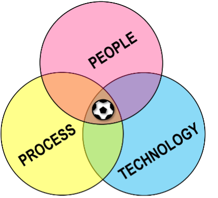
Shown below is the well-known ‘People-Process-Technology’ framework, first published by Leavitt (1964). In this framework, the presence of all three components is critical, as is balance between them – sometimes referred to as the ‘sweet spot’ or ‘golden triangle’. I have found this balance to be a critical success factor for any assurance or peer-review process. Let’s look at each component as they relate to prospect peer review and assurance.
Prospects are based on technical data and the interpretations of those data. In this regard, I consider technology to include not only the acquisition and application of state-of-the-art technology, but also applying ‘technical know-how’ as well as considering the availability and assessment of technical data (these latter two are also dependent on people).
Prospects are all about data and how we interpret that data, and the proper use of statistics to unambiguously characterize the data. However, all this is not done by computers, it’s done by human beings, who apply their expertise to interpretations, judgements, and decisions all along the way—so in the end, prospects are inventions of people.
You can’t have a prospect without physical data to describe it and allow understanding of risks and uncertainties, nor can you have a prospect without a person to aggressively seek all necessary relevant data, make observations, and interpretations. And only humans can properly integrate all the pieces of technology and quantification, all the while making judgements under conditions of uncertainty. Furthermore, a prospect is only as good as the prospector’s technical abilities, intuition, and objectivity, so this component relies heavily on the experience and training of your staff. Finally, prospects do not have feelings, but people do, and recognizing and respecting that all prospects are ‘someone’s baby’ is a make-or-break aspect of assurance.
Underlying any E&P decision is the process that results in that decision. Subsurface excellence depends on having a consistent and well-understood process. It has been well-demonstrated that exploration success starts with selecting the best prospects from an inventory (Pettingill, 2005). That in turn requires discipline and consistency within the selection process. Equally important is the learning process and associated predictive performance tracking, which provide the foundation of positive change. Finally, a process is only sound when it is communicated effectively and transparently to those who must follow it (back to people!). In this regard, simplicity is a great friend.
Now let’s look at what happens when our diagram lacks balance.
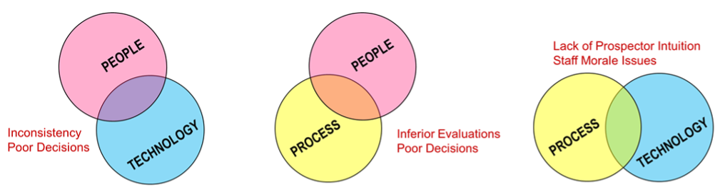
This results in inconsistency which by itself usually leads to poor project selection, continued pursuit of inferior prospects (which burns resources!) and finally inhibits organizational learning. Another aspect that can be lost is diversity of opinions, which reduces bias and often launches healthy debates that identify issues that would otherwise be missed. Often this results in dry holes.
When the underlying technology, understanding of it, or application of it is not sound, the final evaluation product (upon which decisions are made) will be inferior and unsound. More dry holes!
This leads to a host of issues, both short-term and long-term. In the immediate term, peer review meetings can become mechanical, which in turn have several effects: 1) the intuition of the subsurface professionals is not captured, 2) the meeting can have a backdrop of fear, hostility, reluctance to share thoughts, or even 3) tactics that ultimately undermine the process. Longer term effects can set in, such as lack of confidence in the assurance process (or even resentment of it) and staff morale issues – even to the point of causing staff attrition and with it, loss of subsurface ‘know-how’ and excellence. More dry holes!
Have you ever witnessed examples of these three ‘imbalance’ scenarios? I certainly have, and in every case, they resulted in an unfortunate decision that I wish I had not been a part of. In more than one case, a dry hole resulted that I realized should not have been drilled.
In summary, if our assurance process is to succeed, we must hit the sweet spot of People, Process and Technology. If we fail to concentrate on all three, it will be very difficult for us to achieve sustained excellence.
The next article in the series, contributed by James Handschy who was responsible for the subsurface Assurance process at ConocoPhillips, will address how corporate culture can influence the assurance process.
Leavitt, H. J., 1964, Applied Organization Change in Industry: structural, technical and human approaches. In W. Cooper, H. J. Leavitt & M. W. I. Shelly (Eds.), New Perspectives in Organization Research, pp. 55-71, New York: John Wiley.
Pettingill, H.S., 2005, Delivering on exploration through Integrated portfolio management: The whole is not just the sum of the holes, SPE AAPG Forum, Delivering E&P Performance in the Face of Risk and Uncertainty: Best Practices and Barriers to Progress. Galveston, Texas, Feb. 20-24, 2005.
Henry was the head of technical assurance for Repsol from 1996 until 2000, and for Noble Energy from 2002 until 2013. He was an Explorationist with Shell, Repsol and Noble for 35 years before joining Rose & Associates in 2018, where his primary role is chairman the company’s DHI Consortium.
by Kenneth C. Hood, Guest Contributor
Part 1 of this discussion illustrated the impact of the approach used to represent candidate hydrocarbon column height distributions and the importance of checking for geologic plausibility. Ideally, this checking should take place prior to any assurance review with an assurance team member who specializes in aspects of seal integrity, but many times that checking is done at the assurance review. The reason the checking is important is because of the dramatic influence the column height can have on prospect metrics. That is the focus of Part 2 of this blog on column height.
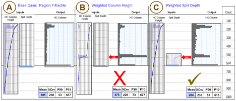
The selected column height (or contact depth) distribution can dramatically impact the volumetric outcomes for an opportunity, and thus on the economic chance of success. The top of the figure 2 (with the depth y axis) illustrates seven alternative column height scenarios (shown as bar frequency and cumulative line frequency displays) applied to the same 500 m relief trap (with a schematic cross section shown on the far left adjacent to the depth axis). The bar chart immediately below shows for each scenario the percent of geologic successes that are economic failures.
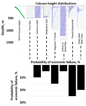
Because the different cases in this example represent the same trap (with a 40% chance of prospect geologic success) with alternative column height distributions, the probabilities of economic failure are based on simple volume thresholds and can vary dramatically based on the input column height distribution (Hood, 2019). Here the filled to spill model has a 100% chance of economic success given geologic success.
Often alternative scenarios will be required for a column height distribution. As an example, it may be necessary to use different column height distributions for oil, multiple-phase, or gas accumulations. Prospects for which a seismic-based Direct Hydrocarbon Indicator (DHI) constrains the potential range of contact depths provide a special case. The seismically constrained contact can be represented as a separate scenario, or as part of a weighted contact distribution. The weight associated with that outcome should be correlated to the DHI chance of validity (the higher the chance of validity, the more weighting can be assigned).
Because of the complexities associated with column height distributions, it is best to avoid using a single deterministic analysis to evaluate the hydrocarbon potential for an opportunity. Using the filled-to-spill case is generally too optimistic for representing opportunities. Generally, a full probabilistic analysis must be created to determine the mean or median column height that would be used in a single representative case.
I thank ExxonMobil for releasing this material. Many colleagues have contributed to this work.
Hood, K., 2019, Hydrocarbon Column Height, Presentation at the 2019 Rose & Associates Risk Coordinators Workshop # 17, Houston, Texas.
Ken Hood holds a Ph.D. in Geology from The University of Kansas. Ken retired in 2020 after 31 years with ExxonMobil. Much of his career was spent working in assessment and assurance of conventional and unconventional resources at play and prospect scales.
by Kenneth C. Hood, Guest Contributor
When geoscientists evaluate an opportunity, we tend to focus on the geological aspects we are most familiar with. This is human nature. Unfortunately, what we spend the most time on may not be the most important factor for understanding an opportunity’s potential. As an example, a team may spend many hours refining estimates of porosity or net-to-gross, when the impact of these parameters often pales in comparison to the impact of hydrocarbon column height (hydrocarbon-water contact depth).
In my assurance experience, different assessment teams have used very different representations of column height or hydrocarbon-water contact depth as part of opportunity evaluations. Often at the screening stage, they would simply evaluate an opportunity as being filled to spill. This, coupled with permissive structure sizes based on preliminary mapping of limited data, tends to result in exceptionally optimistic hydrocarbon volume estimates that almost always get reduced with additional work. Other assessors preferred an exponential decline of column heights from the assessment minimum down to synclinal spill. This would imply that every trap is almost always significantly underfilled, with essentially no chance of being filled to spill. Compared to a filled-to-spill scenario, this is a very pessimistic outlook indeed. While it is important to be as accurate as possible with column height estimates, it is also important to be consistent among opportunities, so they at least have a reliable basis for comparison.
As part of the assurance process, it is essential to verify and document assumptions about seal capacity as well as all potential geometric limits, aka leak mechanisms (including probability), and to ensure that the assessment analysis is created in a manner consistent with the geologic concept being evaluated. Experience has shown that the analyses frequently do not match the geologic description and the available constraints.
The details of how to best represent hydrocarbon column height in an evaluation will vary depending on software capabilities. Where possible, the workflow preferred here is to build background column heights and geometric limits (spill depth) as separate distributions. This approach enables the use of standard background column height distributions for families of related prospects while still honoring the unique configuration of each trap.
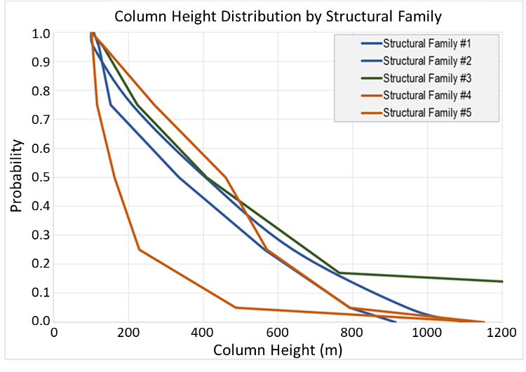
The background column height distribution is the column height supported by bed seal capacity, with a potential overprint of unresolved geometric spills (if based on analogs). Such distributions can be based on capillary constraints (e.g., capillary pressure data coupled with geologic models) or empirical column height data from local or analog discoveries (for a recent example, see Edmundson et al, 2021). Using empirical data can be challenging in that hydrocarbon pools controlled by geometric limits document the minimum column that the seal can support but not the upper limit. Figure 1 illustrates some representative background column height distributions applied to different families of structural prospects. Column height distributions should start at a consistent assessment minimum. The assessment minimum can be effectively linked to seal capacity if based on a minimum column height and not a minimum hydrocarbon volume.
The definable geometric limits on column height include controls such as synclinal spill, reservoir juxtapositions, fault intersections, and channels or scours, each with an associated probability of leak. Each probability is conditional on the success of shallower potential limits, such that the total must sum to 1.0.
Figure 2 illustrates the importance of using separate distributions for column height and geometric limits for an opportunity evaluation. Because the input column height distribution represents the capacity of the seal to support a hydrocarbon column, in many cases it will extend beyond the trap spill(s). During the Monte Carlo convolution, both the column height distribution and the spill depth distribution are randomly sampled. The output column height for each realization is the minimum of these two values, thus creating a mode at the spill limit where the magnitude is automatically scaled to and consistent with the seal capacity. This output distribution is this displayed in a frequency format. In this example, the base case is a 600 m closure with a regional column height distribution, resulting in a mean volume of 305 MOEB (lowermost table, Figure 2A). Now consider the addition of a potential leak, such as a fault intersection, over a 50 m interval centered at 500 m below the crest. This zone has a 0.5 chance of leaking. The realizations for which this leak controls the contact should produce a mode in the output column height distribution. If this mode is represented using a weighted input column height distribution (Figure 2B), the apparent prospect volume actually increases. The increase results because the weighted input distribution reduces outcomes from above the leak as well as below it. Such behavior is not geologic – the leak should only reduce realizations deeper than the fault intersection. By using the regional column height distribution coupled with a weighted spill-depth distribution (Figure 2C), the prospect volume decreases as expected. With the weighted spill distributions, realizations above the leak are unchanged from the base case. This example illustrates how combining the background column height and explicit geometric limit(s) into a single input distribution produces non-geologic and erroneous results in Figure 2B.
Part 2 continues with a discussion of the impact of column height on opportunity evaluation. The impact on the economic viability of an opportunity can be substantial.
I thank ExxonMobil for releasing this material. Many colleagues have contributed to this work.
Edmundson, I.S., Davies, R., Frette, L.U., Mackie, S, Kavli, E.A., Rotevatn, A., Yielding, G, and Dunbar, A., 2021, An empirical approach to estimating hydrocarbon column heights for improved predrill volume prediction in hydrocarbon exploration, AAPG Bulletin v105, n12, pp 2381-2403.
Hood, K., 2019, Hydrocarbon Column Height, Presentation at the 2019 Rose & Associates Risk Coordinators Workshop # 17, Houston, Texas.
Ken Hood holds a Ph.D. in Geology from The University of Kansas. Ken retired in 2020 after 31 years with ExxonMobil. Much of his career was spent working in assessment and assurance of conventional and unconventional resources at play and prospect scales.
By Henry S. Pettingill (with contributions by Roger Holeywell and Rocky Roden)
We have learned quite a lot about Direct Hydrocarbon Indicators (DHIs) in Rose and Associates’ DHI Consortium over the past 23 years. Roger, Rocky and I have generated lots of statistics on successes and failures, and we discuss the learnings from them regularly in our Consortium meetings. In several recent conferences and forums outside the Consortium, however, I have asked: “what do you think the #1 geological outcome is for DHI failures?”
What would your answer be? In every external forum, the first person to shout out the answer has said “LSG”.
First, that the overwhelming #1 cause of false DHIs is wet sand – usually thick and high-quality wet sand. In fact, as you can see from the graph below, over 50% of our failures found wet sands, whereas LSG is tied for #2 with non-reservoirs, 18% each.
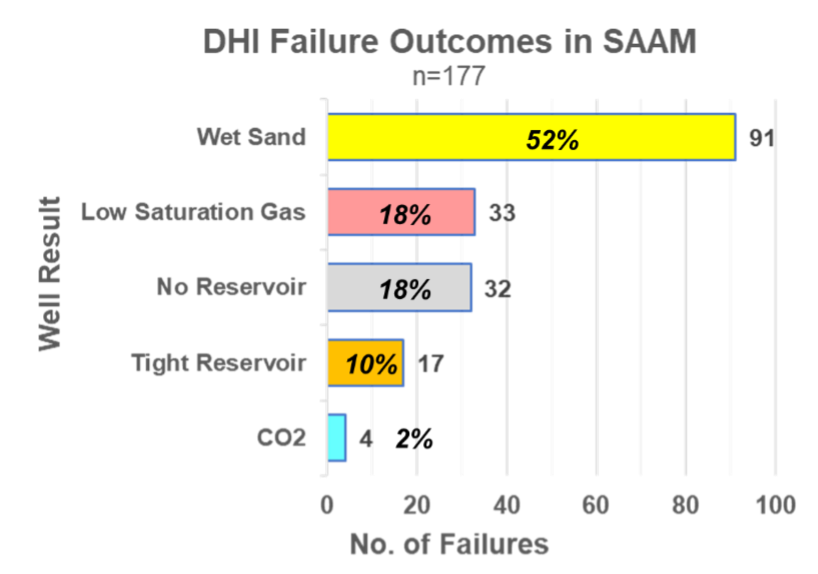
Second, that for 80% of our failures, the anomaly is caused by lithology (wet sand, non-reservoir or tight reservoir). Only 20% are due to fluid effects – 18% from LSG and 2% from CO2 gas.
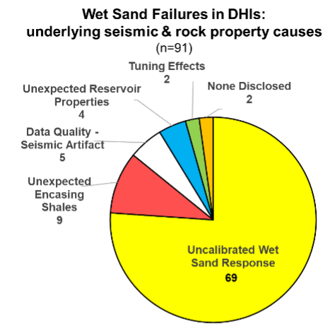
Third, what are the underlying geophysical issues (seismic, rock properties) that can fool us in these wet sand outcomes? The pie chart below addresses this question. As you can see, for three quarters of our wet sand failures, we simply don’t understand how a wet sand response can be reliably distinguished from a fluid effect, most often because of lack of well control or non-uniqueness in the solution space.
1) Do your regional homework, with a rigorous review o well control and well ties. Geologists and Petrophysicists, you have a role to play here! 2) Respect the non-uniqueness of seismic amplitude causes, especially when dealing with seismic models. Avoid confirmation bias and when shown a model match, ask “what else could it be?”. 3) Consider the geophysical pitfalls such as tuning, seismic artifacts, and unexpected reservoir properties, as well as lateral changes in the encapsulating shales that could ‘brighten’ a wet sand.
Acknowledgement: special thanks to the R&A DHI Consortium members and leadership – a group of experts who I am still learning from every day!
References:
Pettingill, H.S., and R. Roden (2022), Integrated DHI Prospect Evaluation: Lessons Learned from Three Generations of Explorers. 2022 IMAGE Conference, Houston, August 19, 2022.
Posted on January 7, 2022 by Lisa Ward
Hello and welcome to Rose & Associates’ blog on Assurance!
By Marc Bond
Collectively Rose & Associates (R&A) has 100 years of experience leading and serving on E&P assurance teams. Along with our many years of consulting and supporting industry assurance teams, R&A is in a unique position to share our learnings and observations on the subject. Our aim is to help improve the effectiveness of assurance and subsequent decision-making, leading to more predictive portfolios.
Throughout this article series, we aim to discuss the concept of exploration assurance, exploring many facets such as the case for assurance, the role of assurance in decision-making, recommended assurance best practices, assurance team behaviors and biases, personal experiences, and pitfalls and challenges. Contributors will include R&A professionals as well as industry leaders experienced with assurance.
We welcome feedback and personal experiences dealing with assurance and encourage you to post your comments.
Assurance describes the process of providing objective, independent, and consistent reality and perspective checks on exploration project characterization. When performed well, it can provide justified confidence to decision-makers in investment decisions and enhance predictive accuracy.
The assurance process begins with a review of a team’s assessment, then the assurance team offers recommendations for further technical work that can clarify the uncertainty, and lastly, all reach a collaborative prediction. Given their independence from the work and wider perspective, the assurance team is not as easily influenced by some of the biases associated with the pride of prospect ownership nor local management influence.
I recently finished reading Kahneman et al Noise: A Flaw in Human Judgment (2021). Since the 1970s Professor Kahneman has established himself as the thought leader on decision theory (including a Nobel prize in Economics), so any book he writes is a must-read when you are in our line of work. Whilst the authors discussed assurance techniques, there was no mention of the concept of assurance. This one practice would have gone a long way in alleviating many of the inconsistent decisions the authors addressed. Frustratingly, there are few peer-reviewed publications covering assurance.
In all instances where judgments and decisions are needed, consistent and predictable outcomes depend upon the accuracy of predictions. Accurate predictions lead to a consistently reliable portfolio, worthy of repeat funding. Left to the individual assessor or team, the predicted outcomes are often inconsistent and inaccurate. The reason for this has many causes, biases being a key component (see attached link to the blog series on bias). The widespread overestimation of resources is a common problem for the oil and gas industry, resulting in loss of value.
Validation of technical assessments by assurance has been shown to contribute to consistent and predictive portfolio management, and thus improved business performance. When done well, assurance will provide additional and diverse perspectives on prospect assessment, share better practices, identify weaknesses in evaluations and assumptions, provide alternatives, and foster consistency. The assurance team should be seen as the ally of the technical team, with a common goal of delivering maximum success from the company’s exploration portfolio.
The assurance process should utilize an integrated approach working with the technical teams to ensure best practices and consistent evaluations. In addition to assistance from staff on the characterization of opportunities, the assurance team will also interact with management to aid in opportunity comparison and support their decision-making.
The following figure outlines the assurance process.
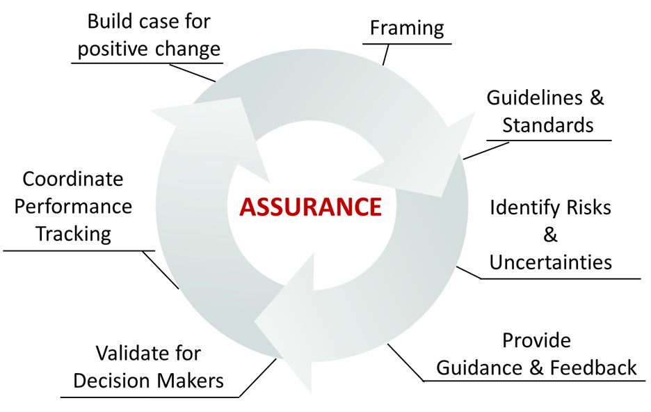
The process starts with the framing of the exploration project to determine the appropriate work program for evaluation. As input into assurance, there should be methods to detect and rectify flaws in analysis and ensure all products (e.g., reservoir models, seismic interpretation and mapping, etc.) adhere to the appropriate standards.
One of the cornerstones of the assurance process is early engagement. The assurance team will consider the key subsurface risks and uncertainties. They will then provide guidance and support to the technical team for best practice pre-drill resource and chance characterization. During the assurance review, the assurance team aims to validate the evaluation (e.g., resource distribution and chance of success), providing confidence to the decision-makers.
After consistency is introduced, calibration comes about from performance tracking, designed to analyze outcomes relative to predictions and capture learnings that feedback in future assessments.
The assurance process should be fit for purpose. Organizations should be clear on what the business requires from assurance, and the process should be designed to deliver these objectives. For all of the stages, there may be multiple cycles depending on the scope and complexity of the project. For example, large complex opportunities typically require several reviews, whereas a small, simple, or inexpensive opportunity may only need a single review.
Whilst these are indeed important considerations, they are not a problem with assurance itself. Any flaws with the design or implementation of the assurance process can all be addressed and alleviated.
Marc was the Subsurface Assurance Manager with BG Group for 6 years, responsible for the company-wide subsurface assurance for all projects, including Exploration, Appraisal and Development ventures and conventional and unconventional resources. He helped create the Risk Coordinators Network in 2008, which remains active. Following the assurance role, he was the Chief Geophysicist at BG.
REFERENCE CITED
Kahneman, Daniel, Sibony, Olivier, and Sunstein, Cass, 2021, Noise: A Flaw in Human Judgment, William Collins, 454p.
This Assurance Blog series is coordinated and edited by Marc Bond, Gary Citron, and Doug Weaver.
Posted on November 10, 2021 by Lisa Ward
By Jim Gouveia, Marc Bond, Jeff Brown, Mark Golborne, Bob Otis, Henry S. Pettingill, and Doug Weaver
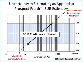
Consider the figure to the right under the lens of predicted net feet of pay. How have you been trained to handle plots such as this one? Here at R&A, we recommend a seven-step approach:
01. Plot the P10 and P90 predictions.
02. Draw a line between the predictions and extrapolate it to the resulting P1 and P99 values.
03. ‘Reality check’ these end members.
On the low end, would the predicted thickness contribute to meaningful sustainable flow? Assuming our area is unknown and highly correlated to our concept of sustainable flow, we get pragmatic and think about the ability to effectively complete the zone, without extraordinary measures. For example, would we be able to effectively complete a 1-foot interval in a homogenous sand which is underlain by 100 ft of water? There is no silver bullet for P99; it will be driven by user experience and play-specific knowledge, with consideration for variables such as permeability, Kv/Kh ratio, depth, infrastructure, viscosity, etc.
One of our biggest challenges when we consider net pay is defining how we differentiate geological successes from commercial successes. (We are talking about the average Net Pay across the productive trap area and not at the planned well location).
On the high end, could one make an optimistic yet realistic prospect map that could house such a thick Average Net Pay? In our collective experience at R&A, the projected P1 value can be unrealistically high—it’s not about the maximum thickness somewhere within the trap, it’s the maximum average thickness across the productive trap area.
04. Adjust the ‘reality check’ high and low members and pragmatically assume these are your new P1 and P99 end members.
05. Plot the ‘reality checked’ P1 and P99 values and redraw the line. The original P10 and P90 values are frequently not preserved and should be thought about as simply serving the purpose of initiating the process. Determine your resulting ‘reality checked’ P10, P50, and P90 values.
06. Inspect your measures of central tendency, the P50, and Mean values. For the P50, ask yourself, “When we think of this prospect, does it feel reasonable that half the time we expect to get a result larger than this value, and half the time less?” In a lognormal distribution, which best characterizes net pay, the P50 is halfway through the frequency, not halfway through the distribution’s parameter values. The Median, which is not synonymous with the P50, is based on sampled data. The reader is advised to always use the P50 which is based on the fitted data. When we are dealing with limited data sets, there can be a significant difference between the Median and the P50.
07. Compare the derived prospect Mean to the distribution of geologically analogous discovered prospects. Predicting a Mean outcome, which lies above the upper ten percent of your analogous discoveries, demands a technically unbiased explanation of why the prospect will have an Average Net Pay that exceeds 90% of the values previously encountered in the play.
Ultimately, exploration organizations need to deliver what they predict, and numerous industry look-back studies have demonstrated that the approach outlined in this example is highly effective in achieving that goal.
The values within our ‘reality checked’ P10 and P90 outcomes represent an “80% confidence interval.” In the E&P industry, we advocate setting the goal for our predictions based upon that range, particularly for the performance of our portfolios (more on that in a later R&A blog).
In a future blog, we will address measures of uncertainty and discuss reality checks based on our ratio of the P10 to P90.
Posted on September 23, 2021 by Lisa Ward
By Jim Gouveia, Marc Bond, Jeff Brown, Mark Golborne, Bob Otis, Henry S. Pettingill, and Doug Weaver
Few industries are fraught with more uncertainty than prospect exploration in E&P. Our formal education guided us with the notion that unless we provide a precise answer, we have ‘failed’ to meet expectations. This is exasperated by investor and leadership’s need for certainty in their investment decisions. When we face an uncertain prediction, we need methods that decouple our minds from trying to jump to ‘the answer’ and instead capture a pragmatic range of possible outcomes.
The present value of our drilling prospects is primarily driven by their probability of realizing commercial success, our corporate discount rate, commodity prices, capital expenses, operating expenses, and our share of the commodity’s cash flow after taxes and royalties. Each of these key parameters is riddled with uncertainty throughout a project’s lifetime.
Modeled ranges better inform decision-makers by fairly representing the spectrum of possible outcomes. Many experts argue that decision-makers simply require confidence in the mean outcome. Portfolio theory advises that given a great number of repeated trials and an unbiased estimation, our firms will deliver the aggregated mean outcome. Whilst portfolio theory is sound, it presupposes two realities that do not exist in the world of exploration. First, our predictions are free of bias. Without a probabilistic basis, grounded by ‘reality checks,’ our forecasts have repeatably proven to be optimistically biased. Second, that there are enough repeated trials to make the aggregate prediction valid over time. No one (especially currently) is drilling enough exploration wells to support high statistical confidence in a program’s ability to deliver a mean outcome.
As decision-makers, we need standardized evaluation techniques upon which we can confidently make our best business investment decisions. That requires that subjective words and phrases such as ‘good chance,’ ‘most likely,’ ‘excellent,’ ‘low risk’ and ‘high confidence’ be eradicated from our presentation of E&P opportunities and replaced with probabilities that have a common definition across all disciplines and projects. The traditional industry consensus is the use of P10 and P90, which in the predominantly used ‘greater than’ convention, represents our optimistic but reasonable high side and our pessimistic but reasonable low side values respectively.
In a prior blog, we introduced our industry-standard method of providing ’P90’ and ‘P10’ values to bracket the ranges of all possible prediction outcomes. Studies have consistently shown that we are not particularly good at making such predictions and tend to underestimate the uncertainty in what we are assessing. For most E&P parameters, this presents itself as having our P10 to P90 ranges too narrow and optimistically high. Until the Petroleum Resources Management System (PRMS) update in 2010, industry guidance for validation of a probabilistic distribution was for the user to compare their probabilistically derived P50 to their deterministic (based upon their best guess) P50. It should not come as a surprise to learn that early probabilistic methods were flawed, as they were based on the belief that in the face of all the inherent subsurface uncertainty, we as subsurface professionals (even those of us who were newly graduated) had an innate ability to directly estimate a P50. Unfortunately, this antiquated belief persists to this day.
So how do we better derive our probabilistic ranges? Let us first bear in mind that we are trying to pragmatically capture the full range of possible outcomes in our predictions. We know that many of our subsurface distributions are often best represented by normal or lognormal distributions. We also know that both normal and lognormal distributions go to positive infinity and that an infinite reserve or rate is neither possible nor pragmatic. On the low end, lognormal distributions approach zero and normal distributions go to negative infinity. At the high end, both lognormal and normal distribution go to infinity. As we are building a distribution to characterize a geological success, we can eliminate the known low and high ends of both distributions either by truncation of outcomes above and below certain thresholds, or our preference at R&A, spike bounding. In spike-bounded distributions, randomly sampled values in excess of the selected high-end limit or low-end limit are respectively set as equal to the selected high- and low-end boundary values. As such the values are ‘bounded’ at the low and high ends of the distribution.
In the exploration realm, we are dealing with a relative dearth of data. Industry experience shows that in the “Exploration space,” we can use the P1 and P99 values of our distributions as the pragmatic end members for our distribution. In practice, we estimate our P90 and P10 values. We then extrapolate these values to a P99 and P1 value. We try to ensure that the P99 value represents the smallest meaningful result – the minimum geological success value – and the P1 value represents the largest geologically defensible result. Our P1 and P99 values are intended to represent a blending of geologic pragmatism and conceptualization. It is a trivial academic debate as to whether these high-end members are or should be our P2, P3 or P0.05 outcomes, the same logic applies to the low-end P99. The use of P1 and P99 should be thought of as a pragmatic spike bounding of the end members (‘reality checks’) of our input distributions.
In summary, our input ranges must capture the entire range of possible outcomes, and industry experience has taught us that to effectivity capture that range, we should consistently employ specifically defined low-side and high-side inputs (e.g., P99, P90, P1, and P10)
In our next article in this series, we will work through an example which addresses Average Net Pay.
Posted on June 11, 2021 by Lisa Ward
by Gary Citron, Senior Associate
“It is amazing what you can accomplish if you do not care who gets the credit.” –Harry Truman
In any successful business, some individuals make significant contributions but remain out of the spotlight. As R&A’s risk analysis software company transitions to a new generation of products, we cannot move forward without recognizing the immense impact R&A Senior Associate Roger Holeywell had as our chief programmer during our MS Excel-based era (1997 to 2020).
Looking for topical yet practical training around 1994, Marathon’s Roger Holeywell attended the AAPG prospect risk analysis class that Pete Rose, Ed Capen and Bob Clapp taught. After completing this classic course, Roger had an epiphany. Converting the concepts, and formulae to MS Excel over the next few weeks, Roger created what became Marathon’s first standardized prospect characterization software. Roger convinced Marathon to widely distribute the software he built. By 1996 Marathon had a standard, consistent package for their prospects.
By 1995 risk analysis concepts became rooted in many larger companies, who similarly built their software packages. The Amerada-Hess Exploration VP phoned Pete to ask if anyone had built software to apply the concepts taught. Pete approached Mobil, Conoco, and Marathon with that request. In short order, Mobil and Conoco said no, but Roger, after checking with Marathon management, replied “Sure, Marathon will license theirs.” Within a couple of weeks, Marathon received $10,000 from Hess, and Hess was a happy client with a new software tool. A couple of months later, Roger called Pete to inform him that Marathon no longer wanted to directly sell software but was willing to partner with Pete because of his extensive contacts. A 1997 contract between Marathon and Pete’s LLC, Telegraph Exploration, provided for a 50-50 revenue split, with Marathon retaining ownership of the code, and Telegraph handling all business matters. To help manage the growth, Pete approached Roger to run the new software company, Lognormal Solutions (LSi), owned by the newly formed Rose & Associates (R&A) in 2000. Roger declined that offer, as he wanted to focus on progressing his career at Marathon.
However, in what became a win-win situation, Roger expressed interest in continuing to raise the profile of his progeny. By 2001 Roger received written approval from Marathon to work for LSi, further progressing the software, but on his own time (nights, weekends, and selected vacation days). By January 2005, Marathon executed an addendum to the 1997 agreement relinquishing all ownership rights of the software to LSi. Roger’s retirement from Marathon in 2015 allowed him to become a full-time Senior Associate and programmer at R&A.
In addition to the prospect software, Roger also coded the original versions of multiple zone aggregation software. These products evolved into Multi-Zone Master (MZM) and Multi-Method Risk Analysis (MMRA). MMRA and Multi-Zone Master would be bundled with a versatile utility program Roger created (Toolbox) to gather, condition, and analyze data to fashion inputs into MMRA software. The toolbox features myriad curve fitting capabilities and calculation of hydrocarbon fluid expansion and shrinkage attributes.
R&A’s software was particularly attractive to companies of mid-size market capitalization. But to serve smaller companies who wanted a consistent characterization platform to demonstrate their savvy Roger built the Essentials Suite in 2004, which had prospect software with two-zone aggregation capability, limited data plotting, and a portfolio aggregator. A much lower price point with basic capabilities admirably serves these smaller companies.
How did all this work get done essentially through one person who worked as a full-time Marathon employee? The answer is PWP (Pajama Weekends Programming). While at home over the weekends Roger’s attire was strictly unadulterated pajamas-only. The design and programming sessions were hardly a picnic, as Roger shared some of the major challenges they tackled. For example, how to keep the software working optimally after Microsoft released versions of Excel that conflicted with the code to create pervasive security or performance issues? Roger experienced one of his most gratifying programming moments in 2005, harnessing Microsoft’s VBA to provide an internal Monte Carlo simulator.
Incredibly, the energy described above that Roger infused into R&A software constituted about 50% of his moonlighting time. The remaining 50%, Roger spent coding SAAM (Seismic Amplitude Analysis Module), the software product generated by R&A’s DHI Consortium. In mid-2000, when many of our clients wanted to see a consistent set of industry-derived best practices around amplitude characterization for chance of success determination (commonly part of ‘risking’), Pete Rose turned to Mike Forrest to geologically weave seismic amplitude anomalies into the fabric of prospect chance characterization. We planned from the start to have Consortium best practices coded into software, so we reached out to Roger to serve as a programmer.
For SAAM, Roger programmed an innovative interrogation process that facilitates a systematic and uniform grading of the amplitude anomaly, beginning with the geologic setting, a preliminary chance assessment solely from geology (Pg), and salient amplitude attributes the seismic survey is designed to extract. SAAM requests the exploration team to answer questions about AVO classification, seismic data quality, rock property analysis, analogs, and potential pitfalls. Thus, SAAM successfully institutionalizes a thorough process they might otherwise avoid or forget. Through the Consortium-derived parameter weighting system, SAAM registers the impact of data quality and seismic observations as well as any rock properties modeling, to determine a modifier to the initial Pg. This modification or ‘Pg uplift’ is now calibrated by over 350 drilled wells. Success rates recorded in SAAM’s database can be critically compared to the forecast success rates to further calibrate the weighting system employed. The Consortium remains a vital industry gathering. Roger attributes longevity to the breakthrough thought that meetings should be member-driven, designed around presentations about a prospect by a member company. During Consortium meetings Roger populates a SAAM file for each prospect in real-time during the presentation, and then the members discuss if they would drill the prospect guided by the SAAM inputs and outputs. Finally, the company reveals the drilling results. All inputs, outputs, and results are added to the database. SAAM’s architecture and workflow were based on a collaborative framework from the very beginning.
It’s hard to fathom the magnitude of such varied software-related contributions built solely in his ‘spare time,’ so for all he has done, here’s a toast to Roger Holeywell, an unsung hero working behind the scenes creating value from risk analysis.
Posted on May 4, 2021 by Lisa Ward
Abridged from a presentation by David Cook and Mark Schneider.
View the original poster
Read the full paper
Rose & Associates introduced the Pwell concept at the AAPG 2017 convention in Houston and released the methodology in our Multi-Method Resource Assessment (MMRA) program in early 2018. This method is now available in RoseRA, our current prospect risk analysis software. The Pwell function in RoseRA provides insights into the balance between the chance of success and the potential resources when a well is drilled in a location that is downdiped from the crest of the structure.
Choosing the best downdip location, giving your discoveries a higher probability of finding Estimated Ultimate Recovery (EUR) hydrocarbons exceeding the Minimum Commercial Field Size (MCFS)
Understanding the impact on the chance of geologic and commercial success
Ensuring that, in the event of a dry hole, there will be “no regrets” about potential up-dip volumes tempting a decision-maker to drill a sidetrack or new well up-dip.
The Pwell function in RoseRA requires that an Area distribution be modeled using either the Area-vs-Depth or Area x Net Pay rock volume estimating methods. Users can input the closing contour area at the proposed well location and simulate it to calculate new metrics for the well location including:
The Pwell chances of geologic and commercial
Given a discovery, the range of resources up-dip and downdip from the well location.
Given a dry hole, the range of “attic” resources up-dip from the well location and the up-dip chance of commercial success.
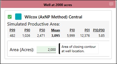
In the following example, the team has proposed a downdip well location at 2,000 acres. The total prospect has a Pg = 50% and a Geologic Mean of 56 mmbo based on an area distribution with P90 of 1,000 acres and P10 of 6,000 acres. The commercial MCFS is 25 mmbo which results in the probability of commercial success being 37.1% and a commercial mean of 70 mmbo. Input the downdip closing contour area of 2,000 acres into RoseRA and run the simulation to observe the results.
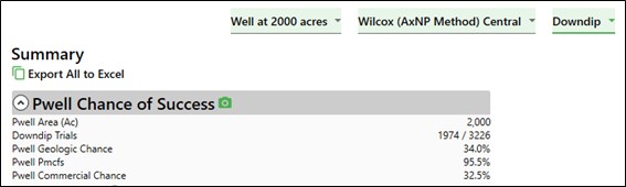
The Pwell chance of success decreases the further downdip the well is drilled. In this example, the Pwell geologic chance of success at the 2,000-acre downdip location is 34.0%, much lower than the crestal Pg of 50%. The tradeoff is that the proportion of the commercial downdip resources is high (95.5%), making the Pwell commercial chance (32.5%) only slightly below the Pwell geologic chance. Given success, you are almost guaranteed a commercial accumulation by drilling at the 2,000-acre location.
There is still the possibility of resources being present up-dip if the well location is dry. What is the commercial chance of success for the potential up-dip resources given a dry hole?
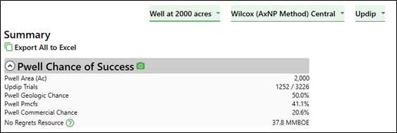
Pg for the up-dip resources remains the same as the original crestal Pg of 50%. About 41% of the up-dip resource distribution exceeds the MCFS so the Pwell commercial chance is 20.6%. Would that Pwell commercial chance tempt management to drill an expensive sidetrack or a second well to determine whether commercial resources are present? Management would need to know the up-dip resource distribution to make an informed decision.
Use Pwell to investigate the up-dip and downdip geologic and commercial resources as shown in the Pwell log probit below.
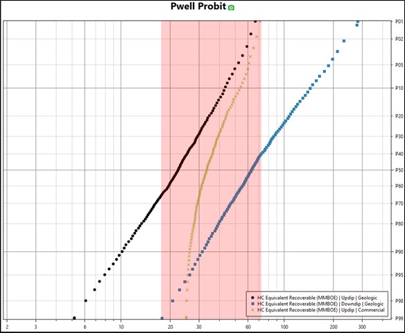
Updip geologic resources (black) range from P99 of 5 mmbo to a P01 of 66 mmbo with a Mean of 25 mmbo. Downdip geologic resources (blue) range from P99 of 18 mmbo to a P01 of 282 mmbo with a mean of 79 mmbo. The red shading indicates the overlap between the up-dip EUR distribution from P65 to P01 and the downdip EUR distribution from P99 to P45. Resources in excess of about 71 MMBO are not achievable in the up-dip EUR distribution. What is the consequence of the distribution overlap region on decision-making?
With the commercial MCFS of 25 mmbo, the up-dip commercial resources (green) show the up-dip Pmcfs is 41.1% and the up-dip Pc is 20.6%. This commerciality possibility might tempt management to spend additional capital to test for an up-dip commercial accumulation. If this is the case, perhaps the well should be drilled further up-dip to minimize total drilling capital.
Another metric that has been used in the industry to gauge whether or not to spend additional capital is the “No Regrets” resource, which is calculated as the up-dip productive area above the drilled location multiplied by the up-dip mean net pay and the up-dip mean oil yield. Figure 5 shows the “No Regrets” resource is 38 mmbo. Notice that this method provides a deterministic value to aid in decision-making instead of the full up-dip distribution and additional insight that RoseRA provides.
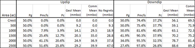
RoseRA provides the ability to model multiple zones, multiple wells, and multiple downdip Pwell areas, shown as vertically stacked zones in a single file. It simulates and reports all entities within the same simulation. Figure 5 shows the up-dip and downdip chances and EURs as increments from the crest to 2,500 acres. Determine which downdip location balances risk, volume, and value for your company.
The RoseRA Pwell function reports clear tabular and graphical outputs so that the rationale for drilling the exploration well downdip can be discussed and communicated with team members and management. Pwell helps facilitate the chance of making a commercial discovery while minimizing the need to spend additional exploration capital. Such scenarios might involve drilling a downdip appraisal well to confirm commerciality, or in the event of a dry hole, avoid drilling an up-dip sidetrack or additional well to determine whether there is a “left-behind attic” resource. A dry hole with the potential for up-dip commercial EUR creates a real conundrum. The Pwell analysis with up-dip and downdip distributions can help clarify a better decision.
This methodology can also help users select locations for appraisal wells. The only difference from the exploration example above is that the crestal exploration discovery results in a prospect Pg = 100%, and the Pwell analysis is performed using the updated resources distribution following the discovery well.
Contact Phil Conway and David Cook at Rose & Associates today to get a demo or more information.
The implementation of Pwell in RoseRA is built on the methodology described in the following reference:
Schneider, F. M., Cook, D. M., Jr. (2017, April 2-5), Drilling a Downdip Location: Effect on Updip and Downdip Resource Estimates and Commercial Chance [Poster session], AAPG 2017 Annual Convention, Houston, TX, United States.
http://www.searchanddiscovery.com/documents/2017/42102schneider/ndx_schneider.pdf
Posted on April 26, 2021 by Lisa Ward
by Creties Jenkins, Partner at Rose & Associates
Take 30 seconds to memorize these 10 items from a shopping list, and then write down how many you can recall: milk, yogurt, croissants, bananas, muffins, coffee, ham, jelly, cheese, and eggs. Most people will be able to remember about 7 items. Now make a note to construct this list again from memory in 24 hours. How many do you think you’ll recall? I’ll be impressed if you can list 5 or more!
The problem, of course, is that this list is being held in your short-term memory (STM) and doesn’t get transferred to long-term memory (LTM). As you can see, STM has a severe capacity limitation. However, this can be overcome, in part, by informational grouping. So if you noticed that the list above consists of breakfast items, you can create this organizational structure in your LTM to help you more easily recall the items next time.
This interconnectedness of information is a cornerstone of memory. Think of memory as a massive, multi-dimensional web in which data is retrieved by tracing through the network. Retrievability is influenced by the number of storage locations as well as the number and strength of the pathways. The more frequently a path is followed, the stronger the path becomes.
This can be illustrated by comparing the abilities of chess masters and ordinary players. If you randomly place 20-25 chess pieces on a board for 5-10 seconds, each of these groups will only be able to recall the positions of about six pieces. However, if the positions are taken from an actual game, the masters will be able to reproduce nearly all of the positions whereas the ordinary players will still only be able to recall the positions of six pieces.
The masters are using their LTM to connect individual positions into recognizable patterns that ordinary players do not see. This ability to recall patterns that relate facts to each other and broader concepts (such as strategy) is critical for success in chess. But what about the business world?
Decision makers and subject matter experts often see themselves as the equivalent of chess masters. They believe the data and experiences contained in their LTM allow them to uniquely perceive patterns and draw inferences that give them a competitive advantage. What’s forgotten many times, is that unlike chess, the permissible moves in the oil and gas business are constantly changing.
Once you start thinking about a given challenge, the same pathways that led you to a successful outcome in similar challenges will get activated and strengthened. This can create mental ruts that make it difficult to process different perspectives, including those that could lead to a better outcome. Our memories are seldom reassessed or reorganized in response to new information, making it difficult to modify these existing patterns.
To overcome this, you need a wider variety of patterns to reference and greater processing of new information to fully understand its impact. This means reaching out to a wider network of experts and devoting more time and effort to develop a deeper understanding, as well as implementing procedures that facilitate this including framing sessions, peer reviews, and performance lookbacks.
These procedures, as well as others, are discussed and practiced in our Mitigating Bias, Blindness and Illusion in E&P Decision Making course. Please consider joining us for a virtual or in-person offering, either as an open enrollment or internal session at your company.
Reference excerpted for this blog: Heuer, Richard J., Jr., 1999, Psychology of Intelligence Analysis, Center for the Study of Intelligence.